<![CDATA[adereth]]>2021-08-01T12:38:01-07:00http://adereth.github.io/Octopress<![CDATA[Distributed Black-Box Optimization Talk at QCon]]>2018-01-03T10:16:00-08:00http://adereth.github.io/blog/2018/01/03/distributed-black-box-optimization-talk-at-qconnyHimmelblau’s Function, a popular test function for black-box optimization
I gave a talk on Distributed Black-Box Optimization at QCon NY 2017. The video and slides are available here.
For reference, here are all the papers that are mentioned in the talk in the order they are covered:
]]><![CDATA[Playing with Wolfram Playing Cards]]>2017-11-02T14:10:00-07:00http://adereth.github.io/blog/2017/11/02/playing-with-wolfram-playing-cardsA few weeks ago, I knocked my favorite mug off the counter and it shattered. RIP:
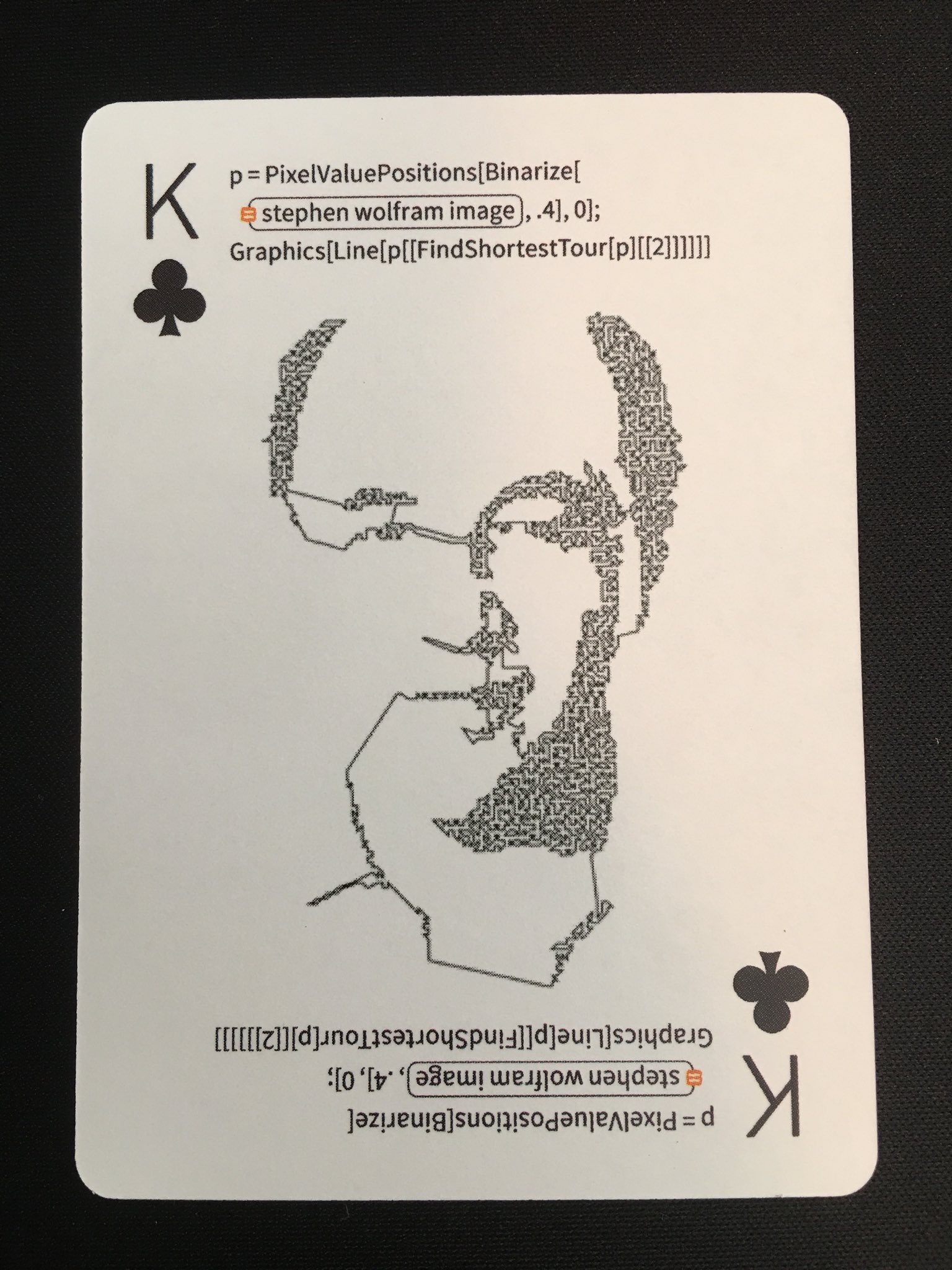
Like a good consumer, I immediately went to the Wolfram store to buy a replacement, but they no longer make it. They did have a deck of playing cards which promised a unique illustration and generating code on each card. How could I pass it up?
The cards arrived a few days ago and they were way cooler than I imagined. As I flipped through the deck, I realized a lot of the cards would be really interesting as starting points for animations. I’ve been going to town with them and posting to Twitter in an epic thread.
4♥️ (Hot take: this is surprisingly bad code. Side effects? Unnecessary call to Image in the loop? Should be a single expression!) pic.twitter.com/XsJUHM67El
Thanks for making it this far! Your reward is the K♣:
]]><![CDATA[Writing a Halite Bot in Clojure]]>2016-12-06T10:42:00-08:00http://adereth.github.io/blog/2016/12/06/writing-a-halite-bot-in-clojure
Halite is a new AI programming competition that was recently released by Two Sigma and Cornell Tech. It was designed and implemented by two interns at Two Sigma and was run as the annual internal summer programming competition.
While the rules are relatively simple, it proved to be a surprisingly deep challenge. It’s played on a 2D grid and a typical game looks like this:
Each turn, all players simultaneously issue movement commands to each of their pieces:
Move to an adjacent location and capture it if you are stronger than what’s currently there.
Stay put and build strength based on the production value of your current location.
When two players’ pieces are adjacent to each other, they automatically fight. A much more detailed description is available on the Halite Game Rules page.
Bots are run as subprocesses that communicate with the game environment through STDIN and STDOUT, so it’s very simple to create bots in the language of your choice. While Python, Java, and C++ bot kits were all provided by the game developers, the community quickly produced kits for C#, Rust, Scala, Ruby, Go, PHP, Node.js, OCaml, C, and Clojure. All the starter packages are available on the Halite Downloads page.
Clojure Bot Basics
The flow of all bots are the same:
Read the initial state (your player ID and the starting game map conditions)
Write your bot’s name
Read the current gam emap
Write your moves
GOTO #3
The Clojure kit represents the game map as a 2D vector of Site records:
A simple bot that finds all the sites you control and issues random moves would look like this:
123456789101112131415161718
(ns MyBot(:require[game][io])(:gen-class))(defn random-moves"Takes your bot's ID and a 2D vector of Sites and returns a map from site to direction"[my-idgame-map](let [my-sites(->>game-mapflatten(filter #(= (:owner%)my-id)))](zipmap my-sites(repeatedly#(rand-nthgame/directions)))))(defn -main[](let [{:keys[my-idproductionswidthheightgame-map]}(io/get-init!)](println "MyFirstClojureBot")(doseq [turn(range)](let [game-map(io/create-game-mapwidthheightproductions(io/read-ints!))](io/send-moves!(random-movesmy-idgame-map))))))
]]><![CDATA[Bag of Little Bootstraps Presentation at PWL SF]]>2016-04-19T20:25:00-07:00http://adereth.github.io/blog/2016/04/19/presentation-on-the-bag-of-little-bootstraps-at-papers-we-love-tooI recently gave a talk on the Bag of Little Bootstraps algorithm at Papers We Love Too in San Francisco:
My part starts around 31:27, but you should watch the excellent mini talk at the beginning too! For reference, here are all the papers that are mentioned in the talk:
Also, in case there’s any confusion, I don’t train Arabian horses.
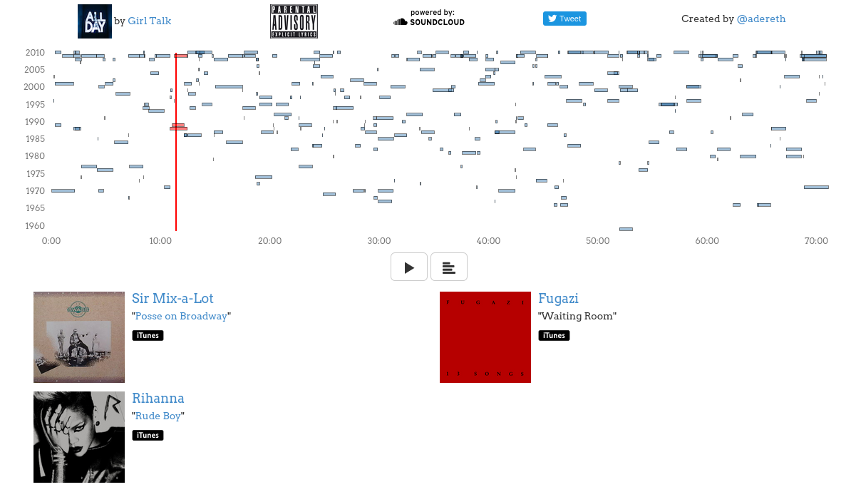
]]><![CDATA[Visualizing Girl Talk: Parsing with Clojure's Instaparse]]>2016-01-20T06:10:00-08:00http://adereth.github.io/blog/2016/01/20/visualizing-girl-talk-with-clojure-and-d3-dot-jsGreg Gillis, also known as Girl Talk, is an impressive DJ who creates mega-mashups consisting of hundreds of samples. His sample selections span 7 decades and dozens of genres. Listening to his albums is a bit like having a concentrated dump of music history injected right into your brain.
I became a little obsessed with his work last year and I wanted a better way to experience his albums, so I created an annotated player using Clojure and d3 that shows relevant data and links about every track as it plays:
I have versions of this player for his two most recent albums:
Unfortunately, they only really work on the desktop right now.
Parsing Track Data
I’ve released all the code that I used to collect the data and to generate the visualizations, but in this post I’m just going to talk about the first stage of the process: getting the details of which tracks were sampled at each time.
There’s an excellent (totally legal!) crowd-sourced wiki called Illegal Tracklist that has information about most of the samples displayed like this:
At first, I used Enlive to suck down the HTML versions of the wiki pages, but I realized it might be cleaner to operate off the raw wiki markup which looks like this:
I wrote a few specialized functions to pull the details out of the strings and into a data structure, but it quickly became unwieldy and unreadable. I then saw that this was a perfect opportunity to use Instaparse. Instaparse is a library that makes it easy to build parsers in Clojure by writing context-free grammars.
Here’s the Instaparse grammar that I used that parses the Illegal Tracklists’ markup format:
The high level structure is practically self-documenting: each line in the wiki source is either a title track line, a sample track line, or a blank line and each type of line is pretty clearly broken down into named components that are separated by string literals to be ignored in the output. It does, however, become a bit nasty when you get to the terminal rules that are defined as regular expressions. Instaparse truly delivers on its tagline:
What if context-free grammars were as easy to use as regular expressions?
The only problem is that regular expressions aren’t always easy to use, especially when you have to start worrying about not greedily matching the text that is going to be used by Instaparse.
Some people, when confronted with a problem, think “I know, I'll use Instaparse.” Now they have three problems. #clojure
Despite some of the pain of regular expressions and grammar debugging, Instaparse was awesome for this part of the project and I would definitely use it again. I love the organization that it brought to the code and the structure I got out was very usable:
]]><![CDATA[Clojure/conj Talk on 3D Printing Keyboards]]>2015-11-19T15:05:00-08:00http://adereth.github.io/blog/2015/11/19/clojure-slash-conj-talk-on-3d-printing-keyboardsI gave a talk on building an ergonomic keyboard using Clojure at Clojure/conj 2015:
Here’s a complete list of the references from the talk, in order of appearance:
]]><![CDATA[Presentation on The Mode Tree at Papers We Love Too]]>2015-04-06T20:10:00-07:00http://adereth.github.io/blog/2015/04/06/presentation-on-the-mode-tree-at-papers-we-love
I did the entire presentation as one huge sequence of animations using D3.js. The Youtube video doesn’t capture the glory that is SVG, so I’ve posted the slides.
I also finally got to apply the technique that I wrote about in my Colorful Equations with MathJax post from over a year ago, only instead of coloring explanatory text, the colors in the accompanying chart match:
Any questions or feedback on the presentation are welcome… thanks!
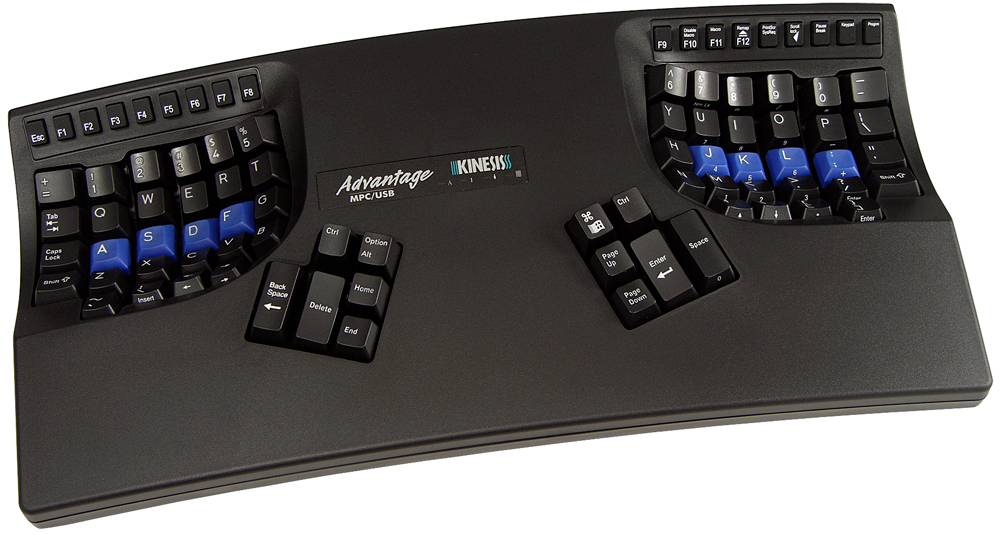
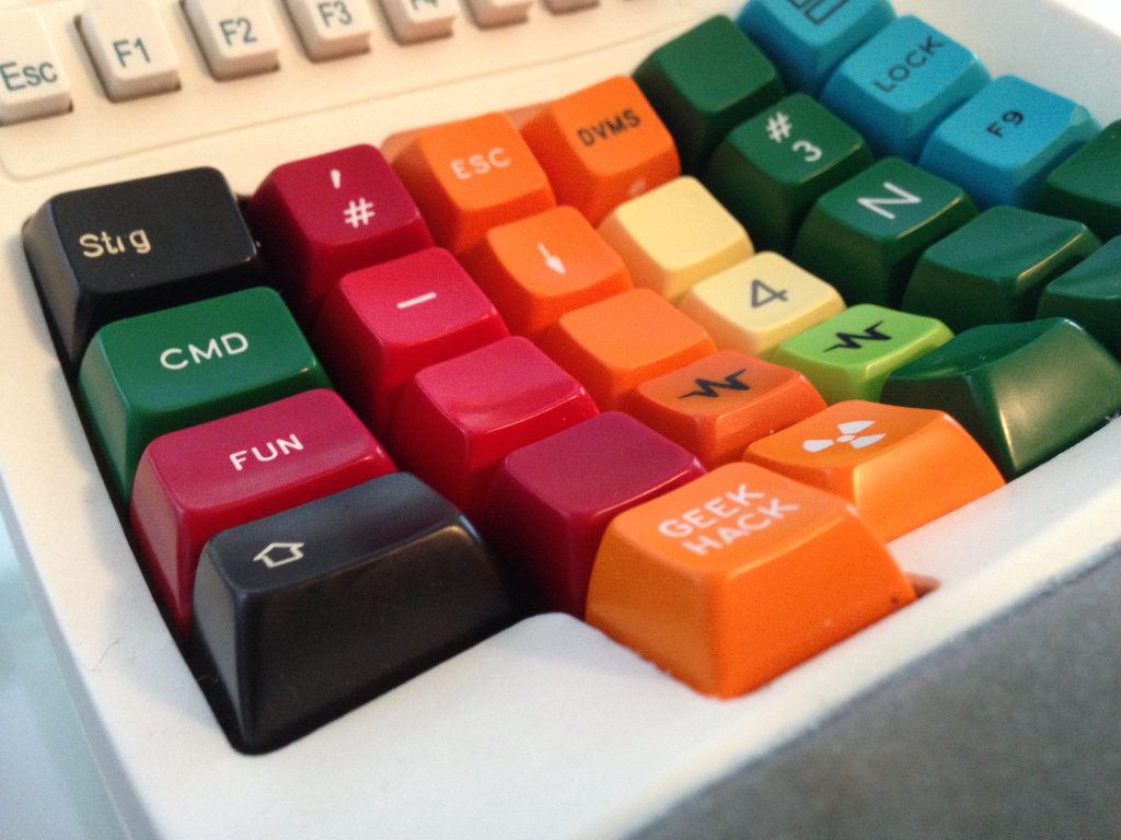
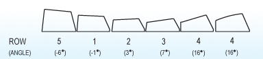
]]><![CDATA[SA Profile Keys on a Kinesis Advantage]]>2015-02-17T16:50:00-08:00http://adereth.github.io/blog/2015/02/17/sa-profile-keys-on-a-kinesis-advantageDespite investingsignificanttime into the Ergodox, I still prefer the Kinesis Advantage:
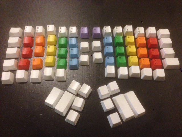
I’ve been (slowly) working on building my own dream keyboard, but in the meantime I make the occasional ridiculous tweak to my Kinesis. This weekend I got 3 lbs. of reject keys from Signature Plastics and I was fortunate enough to get enough keycaps to try something that I’ve been wanting to test for a while.
They are particularly well suited for non-standard keyboard layouts, like the ErgoDox or Kinesis Advantage, because most other keycaps have variable heights and angles that were designed for traditional staggered layouts on a plane.
SA keycaps
Personally, I’m a big fan of the SA profile:
They’re super tall and are usually manufactured with thick ABS plastic and given a smooth, high-gloss finish. I’m a bit of a retro-fetishist and these hit all the right spots. It’s no surprise that projects and group buys that use SA profile often have a retro theme:
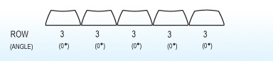
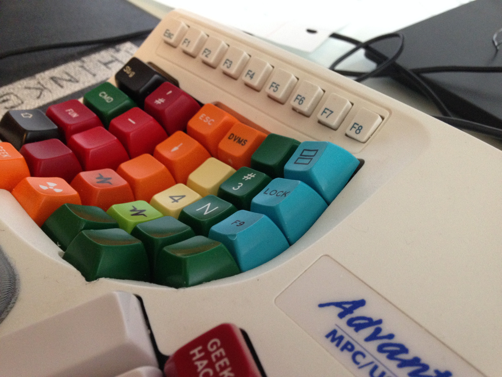
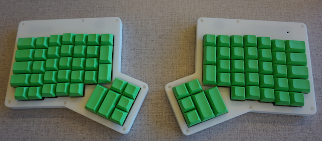
For this project I decided to go with all Row 3 profile SA keys in the two main key wells. Row 3 is the home row on traditional layouts and the keycaps are completely symmetric, just like the DSA profile keys. I was concerned about two main things:
The curvature of the key well combined with the height might mean that the keys hit each other towards the top.
Jesse ran into one spot in the corner of the keywell closest to the thumb clusters where the keycap hit the plastic. This would almost certainly be a problem with the much larger SA keys.
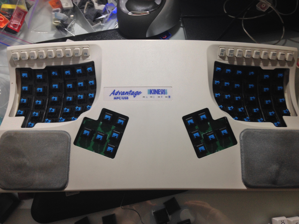
The easiest way to find out was to pop off all the keycaps:
…and to see what fit:
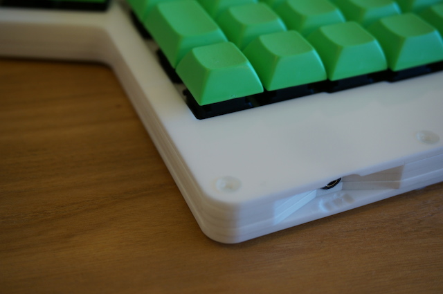
Fortunately, the height was not an issue. The angles are all perfect and the top of the keys form a relatively tight surface. The smaller gaps between the tops combined with the extreme smoothness of the SA keycaps results in a nice effect where I’m able to just glide my fingers across them without having to lift, similar to the feel of the modern Apple keyboards.
Unfortunately, 3 keys at the bottom of each keywell wouldn’t fit. I busted out the Dremel and carved out a little from the bottom, making room for those beautiful fat caps:
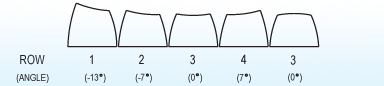
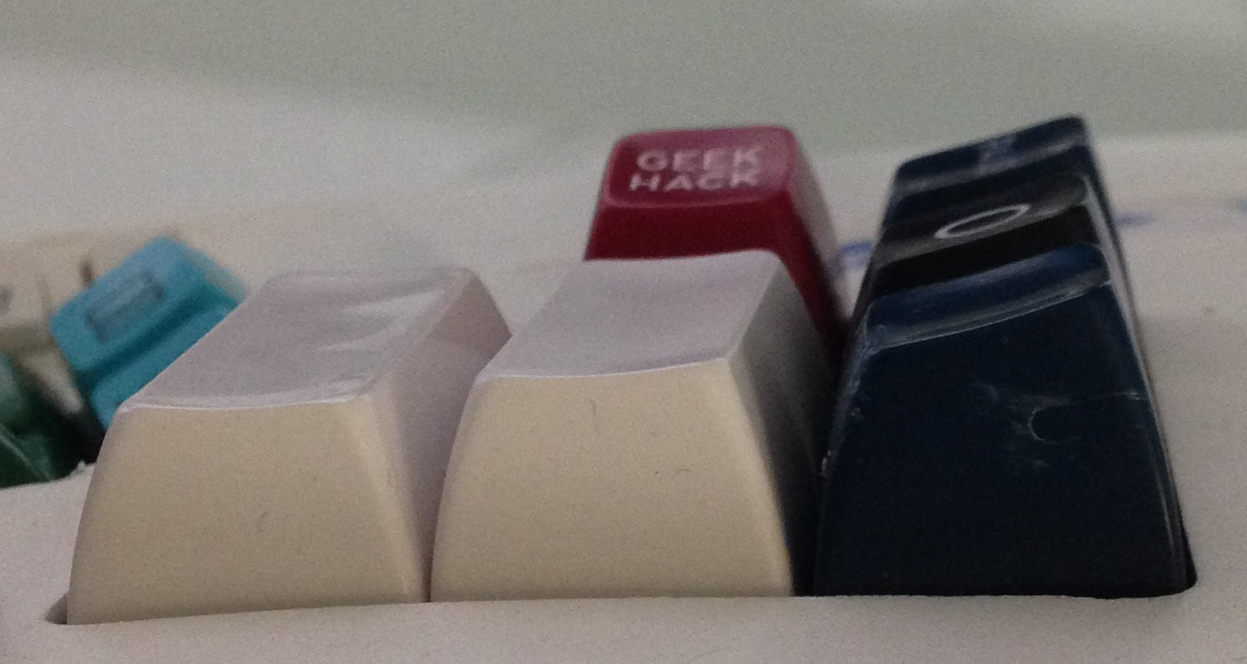
I used Row 1 keycaps for the 1x keys in the thumb clusters. The extra height makes them not quite as difficult to reach:
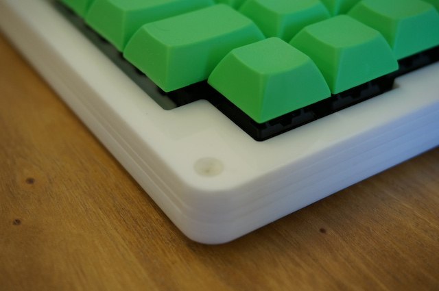
Conclusion
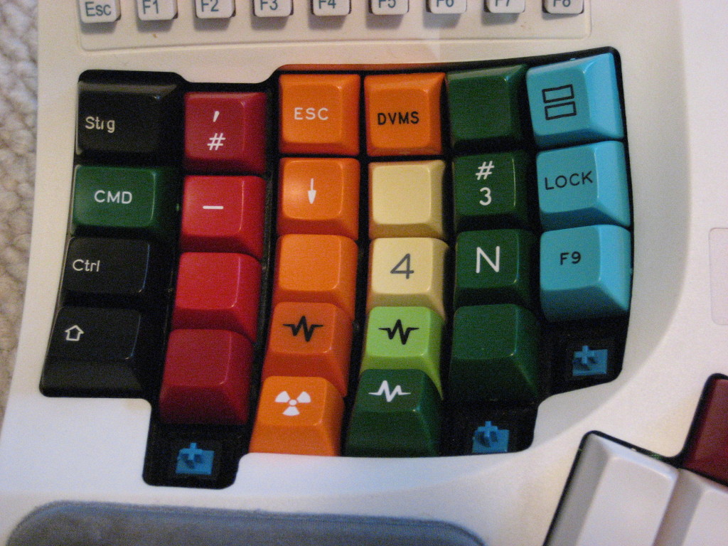
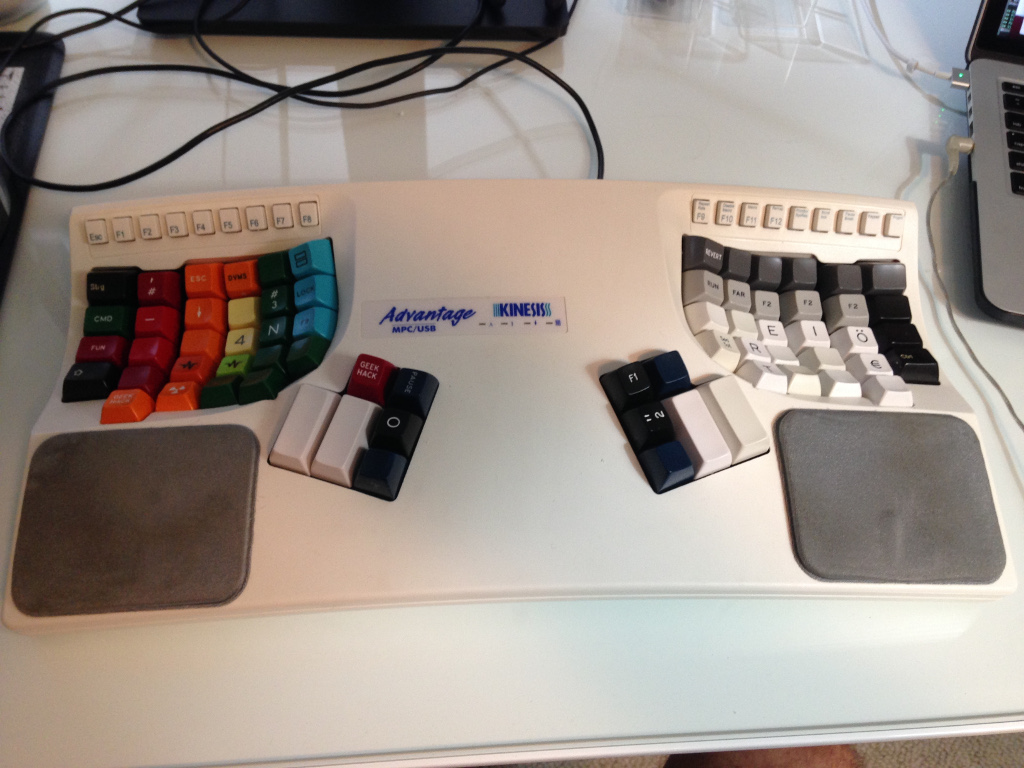
Overall, I’m pretty happy with how it turned out:
It’s a pleasure to type on and I’m convinced that SA profile keys are going to be what I use when I eventually reach my final form.
If you’re interested in doing this yourself, you should know that it’ll be difficult to source the 1.25x keys that are used on the sides of the Kinesis Advantage. A lot of the keysets that are being sold for split layouts are targeting the Ergodox, which uses 1.5x keys on the side. It does look like the Symbiosis group buy includes enough 1.25x’s in the main deal, but you’d need to also buy the price Ergodox kit just to get those 4 2x’s. If you don’t mind waiting an indefinite length of time, the Round 5a group buy on Deskthority is probably your best bet for getting exactly what you want.
]]><![CDATA[Poisonous Shapes in Algebra and Graph Theory]]>2015-02-02T03:10:00-08:00http://adereth.github.io/blog/2015/02/02/poisonous-shapesI recently started learning about Algebraic Lattices because I was interested in how they relate to Automata Theory. It turns out they’re fundamental to a bunch of other things that I’ve always wanted to learn more about, like CRDTs and Type Theory.
I stumbled upon an interesting property about lattices that reminded me of something from Graph Theory…
If $(L, \leq)$ is a partially ordered set, and $S \subseteq L$ is an arbitrary subset, then an element $u \in L$ is said to be an upper bound of $S$ if $s \leq u$ for each $s \in S$. A set may have many upper bounds, or none at all. An upper bound $u$ of $S$ is said to be its least upper bound, or join, or supremum, if $u \leq x$ for each upper bound $x$ of $S$. A set need not have a least upper bound, but it cannot have more than one. Dually, $l \in L$ is said to be a lower bound of $S$ if $l \leq s$ for each $s \in S$. A lower bound $l$ of $S$ is said to be its greatest lower bound, or meet, or infimum, if $x \leq l$ for each lower bound $x$ of $S$. A set may have many lower bounds, or none at all, but can have at most one greatest lower bound.
A partially ordered set $(L, \leq)$ is called a join-semilattice and a meet-semilattice if each two-element subset $\{a,b\} \subseteq L$ has a join (i.e. least upper bound) and a meet (i.e. greatest lower bound), denoted by $a \vee b$ and $a \wedge b$, respectively. $(L, \leq)$ is called a lattice if it is both a join- and a meet-semilattice.
That’s a lot to take in, but it’s not so bad once you start looking at lattices using Hasse diagrams. A Hasse diagram is a visualization of a partially ordered set, where each element is drawn below the other elements that it is less than. Edges are drawn between two elements $x$ and $y$ if $x < y$ and there is no $z$ such that $x < z < y$.
For example, if we define the $\leq$ operator to be “is a subset of”, we get a partial ordering for any powerset. Here’s the Hasse diagram for the lattice $(\mathcal{P}(\{1,2,3\}), \subseteq)$:
In this case, the $\subseteq$ operator results in $\vee$ (the “join”) being union of the sets and $\wedge$ (the “meet”) as the intersection of the sets. It’s a tragic failure of notation that $\vee$ means you should find the common connected element that is above the pair in the diagram and $\wedge$ means you should look below.
Another example is the set of divisors of a number, where the $\leq$ operator means “divides into”. Here’s the Hasse diagram for all the divisors of 30:
In this case, $\vee$ ends up meaning Least Common Multiple and $\wedge$ means Greatest Common Divisor.
Yet another example is the set of binary strings of a fixed length $n$, with $S \leq T$ meaning $S_i \leq T_i$ for $1 \leq i \leq n$:
In this case, $\vee$ is the binary OR operator and $\wedge$ is the binary AND operator.
These examples are interesting because they’re all the same structure! If we can prove a fact about the structure, we get information about all three systems. These happen to be Boolean lattices, which have the distributive property:
$$a \vee (b \wedge c) = (a \vee b) \wedge (a \vee c)$$
$$\forall a, b, c \in L$$
Now here’s the neat part. There are fundamentally only two lattices that aren’t distributive:
The Diamond Lattice
$$a \vee (b \wedge c) \stackrel{?}{=} (a \vee b) \wedge (a \vee c)$$
$$a \vee 0 \stackrel{?}{=} 1 \wedge 1$$
$$a \neq 1$$
…and:
The Pentagon Lattice
$$a \vee (b \wedge c) \stackrel{?}{=} (a \vee b) \wedge (a \vee c)$$
$$a \vee 0 \stackrel{?}{=} 1 \wedge c$$
$$a \neq c$$
Any lattice that has a sub-lattice that is isomorphic to either the Diamond or Pentagon, referred to as $M_3$ and $N_5$ respectively, is not distributive. It’s not too hard to see, just verify that the corresponding elements that violate distribution above will fail no matter what else is going on in the lattice.
The surprising part is that every non-distributive lattice must contain either $M_3$ or $N_5$! In a sense these are the two poisonous minimal shapes: their presence kills distributivity.
This alone seems like a cool little fact, but what struck me was that this isn’t the first time that I’ve seen something like this…
Planar Graphs
In Graph Theory, there’s a property of graphs called planarity. If you can draw the graph without any of the edges crossing, the graph is planar. The Wikipedia page on planar graphs is filled with awesome facts. For example, a planar graph can’t have an average degree greater than 6 and any graph that can be drawn planarly with curvy edges can be drawn planarly with straight edges, but the most famous result concerning planar graphs is Kuratowski’s Theorem:
A finite graph is planar if and only if it does not contain a subgraph that is a subdivision of $K_5$ (the complete graph on five vertices) or of $K_{3,3}$ (the complete bipartite graph on six vertices)
$K_5$, the complete graph on five vertices
$K_{3,3}$, the complete bipartite graph on six vertices
It turns out there are fundamentally only two graphs that aren’t planar! Any graph that “contains” either of these two graphs is not planar and any graph that isn’t planar must “contain” one of them. The meaning of “contains” is a little different here. It’s not enough to just find vertices that form $K_5$ or $K_{3,3}$ with the edges that connect them. What we need to check is if any subgraph can be “smoothed” into one of these two graphs.
For example, this graph isn’t planar because the red vertex can be smoothed away, leaving $K_{3,3}$:
And?
Unfortunately, I’m just learning about lattice theory and I have no idea if there’s any formal connection between these similar concepts. I have found that there is a branch of lattice theory that is concerned with the planarity of the Hasse diagrams, so it’s not like any algebraist hasn’t thought of this before. If anyone has a formal connection or an example of other cases where a pair of structures have this kind of “poisonous” property, I’d love to hear.
You might be interested in the Robertson-Seymour theorem which says that for any graph property that is closed under taking minors there is a finite list of “forbidden minors” or as you call them “poisonous” graphs. Kuratowski’s theorem is one particular example of this.
This relates also to the concept of well-quasi-orders. A quasi-ordered set $(X, \leq)$ is a well-quasi-order if every infinite sequence ($x_1, x_2, …$) with elements in $X$ has some $i < j$ with $x_i \leq x_j$. An equivalent statement of the Robertson-Seymour theorem is that the set of all finite graphs ordered by the minor relation is well-quasi-ordered.
Another example where “forbidden minors” appear is matroids. Matroids also have minors but unlike graphs they are not well-quasi-ordered under the minor relation. However certain minor closed properties do have a finite list of forbidden minors. For example Rota’s conjecture, which was announced to be proven very recently, says that for any finite field the set of matroids that are representable over that field are characterized by a finite list of forbidden minors.
I started digging into the history of mode detection after watching Aysylu Greenberg’s Strange Loop talk on benchmarking. She pointed out that the usual benchmarking statistics fail to capture that our timings may actually be samples from multiple distributions, commonly caused by the fact that our systems are comprised of hierarchical caches.
I thought it would be useful to add the detection of this to my favorite benchmarking tool, Hugo Duncan’s Criterium. Not surprisingly, Hugo had already considered this and there’s a note under the TODO section:
12
Multimodal distribution detection.
Use kernel density estimators?
I hadn’t heard of using kernel density estimation for multimodal distribution detection so I found the original paper, Using Kernel Density Estimates to Investigate Multimodality (Silverman, 1981). The original paper is a dense 3 pages and my goal with this post is to restate Silverman’s method in a more accessible way. Please excuse anything that seems overly obvious or pedantic and feel encouraged to suggest any modifications that would make it clearer.
What is a mode?
The mode of a distribution is the value that has the highest probability of being observed. Many of us were first exposed to the concept of a mode in a discrete setting. We have a bunch of observations and the mode is just the observation value that occurs most frequently. It’s an elementary exercise in counting. Unfortunately, this method of counting doesn’t transfer well to observations sampled from a continuous distribution because we don’t expect to ever observe the exact some value twice.
What we’re really doing when we count the observations in the discrete case is estimating the probability density function (PDF) of the underlying distribution. The value that has the highest probability of being observed is the one that is the global maximum of the PDF. Looking at it this way, we can see that a necessary step for determining the mode in the continuous case is to first estimate the PDF of the underlying distribution. We’ll come back to how Silverman does this with a technique called kernel density estimation later.
What does it mean to be multimodal?
In the discrete case, we can see that there might be undeniable multiple modes because the counts for two elements might be the same. For instance, if we observe:
$$1,2,2,2,3,4,4,4,5$$
Both 2 and 4 occur thrice, so we have no choice but to say they are both modes. But perhaps we observe something like this:
$$1,1,1,2,2,2,2,3,3,3,4,9,10,10$$
The value 2 occurs more than anything else, so it’s the mode. But let’s look at the histogram:
That pair of 10’s are out there looking awfully interesting. If these were benchmark timings, we might suspect there’s a significant fraction of calls that go down some different execution path or fall back to a slower level of the cache hierarchy. Counting alone isn’t going to reveal the 10’s because there are even more 1’s and 3’s. Since they’re nestled up right next to the 2’s, we probably will assume that they are just part of the expected variance in performance of the same path that caused all those 2’s. What we’re really interested in is the local maxima of the PDF because they are the ones that indicate that our underlying distribution may actually be a mixture of several distributions.
Kernel density estimation
Imagine that we make 20 observations and see that they are distributed like this:
We can estimate the underlying PDF by using what is called a kernel density estimate. We replace each observation with some distribution, called the “kernel,” centered at the point. Here’s what it would look like using a normal distribution with standard deviation 1:
If we sum up all these overlapping distributions, we get a reasonable estimate for the underlying continuous PDF:
Note that we made two interesting assumptions here:
We replaced each point with a normal distribution. Silverman’s approach actually relies on some of the nice mathematical properties of the normal distribution, so that’s what we use.
We used a standard deviation of 1. Each normal distribution is wholly specified by a mean and a standard deviation. The mean is the observation we are replacing, but we had to pick some arbitrary standard deviation which defined the width of the kernel.
In the case of the normal distribution, we could just vary the standard deviation to adjust the width, but there is a more general way of stretching the kernel for arbitrary distributions. The kernel density estimate for observations $X_1,X_2,…,X_n$ using a kernel function $K$ is:
Note that changing $h$ has the exact same effect as changing the standard deviation: it makes the kernel wider and shorter while maintaining an area of 1 under the curve.
Different kernel widths result in different mode counts
The width of the kernel is effectively a smoothing factor. If we choose too large of a width, we just end up with one giant mound that is almost a perfect normal distribution. Here’s what it looks like if we use $h=5$:
Clearly, this has a single maxima.
If we choose too small of a width, we get a very spiky and over-fit estimate of the PDF. Here’s what it looks like with $h = 0.1$:
This PDF has a bunch of local maxima. If we shrink the width small enough, we’ll get $n$ maxima, where $n$ is the number of observations:
The neat thing about using the normal distribution as our kernel is that it has the property that shrinking the width will only introduce new local maxima. Silverman gives a proof of this at the end of Section 2 in the original paper. This means that for every integer $k$, where $1<k<n$, we can find the minimum width $h_k$ such that the kernel density estimate has at most $k$ maxima. Silverman calls these $h_k$ values “critical widths.”
Finding the critical widths
To actually find the critical widths, we need to look at the formula for the kernel density estimate. The PDF for a plain old normal distribution with mean $\mu$ and standard deviation $\sigma$ is:
For a given $h$, you can find all the local maxima of $\hat{f}$ using your favorite numerical methods. Now we need to find the $h_k$ where new local maxima are introduced. Because of a result that Silverman proved at the end of section 2 in the paper, we know we can use a binary search over a range of $h$ values to find the critical widths at which new maxima show up.
Picking which kernel width to use
This is the part of the original paper that I found to be the least clear. It’s pretty dense and makes a number of vague references to the application of techniques from other papers.
We now have a kernel density estimate of the PDF for each number of modes between $1$ and $n$. For each estimate, we’re going to use a statistical test to determine the significance. We want to be parsimonious in our claims that there are additional modes, so we pick the smallest $k$ such that the significance measure of $h_k$ meets some threshold.
Bootstrapping is used to evaluate the accuracy of a statistical measure by computing that statistic on observations that are resampled from the original set of observations.
Silverman used a smoothed bootstrap procedure to evaluate the significance. Smoothed bootstrapping is bootstrapping with some noise added to the resampled observations. First, we sample from the original set of observations, with replacement, to get $X_I(i)$. Then we add noise to get our smoothed $y_i$ values:
Where $\sigma$ is the standard deviation of $X_1,X_2,…,X_n$, $h_k$ is the critical width we are testing, and $\epsilon_i$ is a random value sampled from a normal distribution with mean 0 and standard deviation 1.
Once we have these smoothed values, we compute the kernel density estimate of them using $h_k$ and count the modes. If this kernel density estimate doesn’t have more than $k$ modes, we take that as a sign that we have a good critical width. We repeat this many times and use the fraction of simulations where we didn’t find more than $k$ modes as the p-value. In the paper, Silverman does 100 rounds of simulation.
One of the biggest weaknesses in Silverman’s technique is that the critical width is a global parameter, so it may run into trouble if our underlying distribution is a mixture of low and high variance component distributions. For an actual implementation of mode detection in a benchmarking package, I’d consider using something that doesn’t have this issue, like the technique described in Nonparametric Testing of the Existence of Modes (Minnotte, 1997).
I hope this is correct and helpful. If I misinterpreted anything in the original paper, please let me know. Thanks!
]]><![CDATA[Computing the Remedian in Clojure]]>2014-09-29T09:03:00-07:00http://adereth.github.io/blog/2014/09/29/computing-the-remedian-in-clojureThe remedian is an approximation of the median that can be computed using only $O(\log{n})$ storage. The algorithm was originally presented in The Remedian: A Robust Averaging Method for Large Data Sets by Rousseeuw and Bassett (1990). The core of it is on the first page:
Let us assume that $n = b^k$, where $b$ and $k$ are integers (the case where $n$ is not of this form will be treated in Sec. 7. The remedian with base $b$ proceeds by computing medians of groups of $b$ observations, yielding $b^{k-1}$ estimates on which this procedure is iterated, and so on, until only a single estimate remains. When implemented properly, this method merely needs $k$ arrays of size $b$ that are continuously reused.
The implementation of this part in Clojure is so nice that I just had to share.
First, we need a vanilla implementation of the median function. We’re always going to be computing the median of sets of size $b$, where $b$ is relatively small, so there’s no need to get fancy with a linear time algorithm.
Now we can implement the actual algorithm. We group, compute the median of each group, and recur, with the base case being when we’re left with a single element in the collection:
Because partition-all and map both operate on and return lazy sequences, we maintain the property of only using $O(b \log_{b}{n})$ memory at any point in time.
While this implementation is simple and elegant, it only works if the size of the collection is a power of $b$. If we don’t have $n = b^k$ where $b$ and $k$ are integers, we’ll over-weight the observations that get grouped into the last groups of size $< b$.
Section 7 of the original paper describes the weighting scheme you should use to compute the median if you’re left with incomplete groupings:
How should we proceed when the sample size $n$ is less than $b^k$? The remedian algorithm then ends up with $n_1$ numbers in the first array, $n_2$ numbers in the second array, and $n_k$ numbers in the last array, such that $n = n_1 + n_{2}b + … + n_k b^{k-1}$. For our final estimate we then compute a weighted median in which the $n_1$, numbers in the first array have weight 1, the $n_2$ numbers in the second array have weight $b$, and the $n_k$ numbers in the last array have weight $b^{k-1}$. This final computation does not need much storage because there are fewer than $bk$ numbers and they only have to be ranked in increasing order, after which their weights must be added until the sum is at least $n/2$.
It’s a bit difficult to directly translate this to the recursive solution I gave above because in the final step we’re going to do a computation on a mixture of values from the different recursive sequences. Let’s give it a shot.
We need some way of bubbling up the incomplete groups for the final weighted median computation. Instead of having each recursive sequence always compute the median of each group, we can add a check to see if the group is smaller than $b$ and, if so, just return the incomplete group:
For example, if we were using the mutable array implementation proposed in the original paper to compute the remedian of (range 26) with $b = 3$, the final state of the arrays would be:
Array
$i_0$
$i_1$
$i_2$
0
24
25
empty
1
19
22
empty
2
4
13
empty
In our sequence based solution, the final sequence will be ((4 13 (19 22 (24 25)))).
Now, we need to convert these nested sequences into [value weight] pairs that could be fed into a weighted median function:
Instead of weighting the values in array $j$ with weight $b^{j-1}$, we’re weighting it at $\frac{b^{j-1}}{b^{k}}$. Dividing all the weights by a constant will give us the same result and this is slightly easier to compute recursively, as we can just start at 1 and divide by $b$ as we descend into each nested sequence.
If we run this on the (range 26) with $b = 3$, we get:
]]><![CDATA[Typing Qwerty on a Dvorak Keyboard]]>2014-08-14T18:40:00-07:00http://adereth.github.io/blog/2014/08/14/typing-qwerty-on-a-dvorak-keyboard@thattommyhall posted a fun question on Twitter:
If you type your name on a keyboard marked as qwerty but set to Dvorak and keep reinputting what comes out, will it ever say your name?
— !!!!!11111oneoneone (@thattommyhall) July 31, 2014
The best answer was “yes because group theory” and @AnnaPawlicka demonstrated it was true for her name:
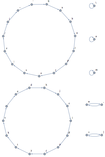
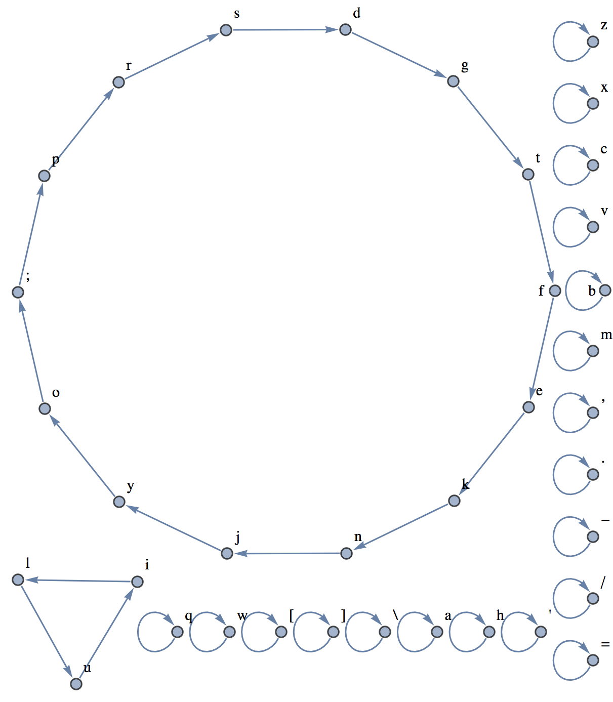
This allows us to visualize the mapping of keys from one layout to another:
1
KeyGraph[dvorak, qwerty]
There is a single directed edge going from each character to the one that will be displayed when you type it. There are 3 keys that remain unchanged, 2 pairs of swapped keys, and 2 large cycles of keys.
\
a
m
] =
, w
. e y t f g u c i d h j k v
[ - ' q p r o l / s n ; z x b
It will take the length of the cycle the letter is in to get the letter we want. For a given word, we won’t get all the letters we want unless we’ve iterated some multiple of the length of the cycles each letter is in. Let’s apply the Least Common Multiple function to see the worst case where there is a letter from each cycle:
]]><![CDATA[Custom Clojure Evaluation Keybindings in Emacs]]>2014-05-29T06:28:00-07:00http://adereth.github.io/blog/2014/05/29/custom-clojure-evaluation-keybindings-in-emacsI love REPL Driven Development. My style is to write expressions directly in the file that I’m working on and to use C-x C-e to view the value of the last command in the minibuffer.
Being able to move my cursor to a sub-expression and see the value of that expression immediately feels like a superpower. I love this ability and it’s one of the things that keeps me locked into Clojure+Emacs as my preferred enviroment.
This power can be taken to the next level by making custom evaluation commands that run whatever you want on the expression at your cursor.
The Basic Pattern
Let’s start by looking at the Elisp that defines cider-eval-last-sexp, which is what gets invoked when we press C-x C-e:
1234567
(defuncider-eval-last-sexp(&optionalprefix)"Evaluate the expression preceding point.If invoked with a PREFIX argument, print the result in the current buffer."(interactive"P")(if prefix(cider-interactive-eval-print(cider-last-sexp))(cider-interactive-eval(cider-last-sexp))))
The important part is that we can use cider-last-sexp to get the expression before the cursor as a string and we can evaluate a string by passing it to cider-interactive-eval. We’ll write some basic Elisp to make a new function that modifies the string before evaluation and then we’ll bind this function to a new key sequence.
If you happen to still be using Swank or nrepl.el, you should use swank-interactive-eval and swank-last-sexp or swank-interactive-eval and nrepl-last-sexp.
Let’s look at some of the useful things we can do with this…
Collections
I frequently deal with collections that are too big to display nicely in the minibuffer. It’s nice to be able to explore them with a couple keystrokes. Here’s a simple application of the pattern that gives us the size of the collection by just hitting C-c c:
If you just use C-c n, Emacs defaults the parameter value to 1. You can pass an argument using Emacs’ universal argument functionality. For example, to get the 0th element, you could either use C-u 0 C-c n or M-0 C-c n.
Write to File
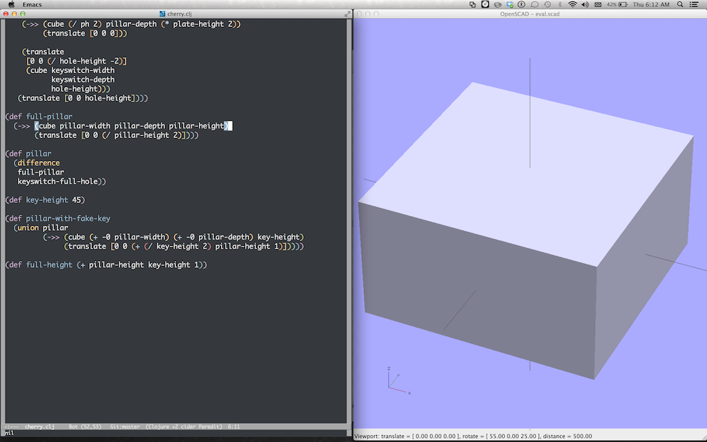
Sometimes the best way to view a value is to look at it in an external program. I’ve used this pattern when working on Clojure code that generates SVG, HTML, and 3D models. Here’s what I use for 3D modeling:
This writes the eval.scad file to the root directory of the project. It’s great because OpenSCAD watches open files and automatically refreshes when they change. You can run this on an expression that defines a shape and immediately see the shape in another window. I used this technique in my recent presentation on 3D printing at the Clojure NYC meetup and I got feedback that this made the live demos easier to follow.
Here’s what it looks like when you C-c 3 on a nested expression that defines a cube:
View Swing Components
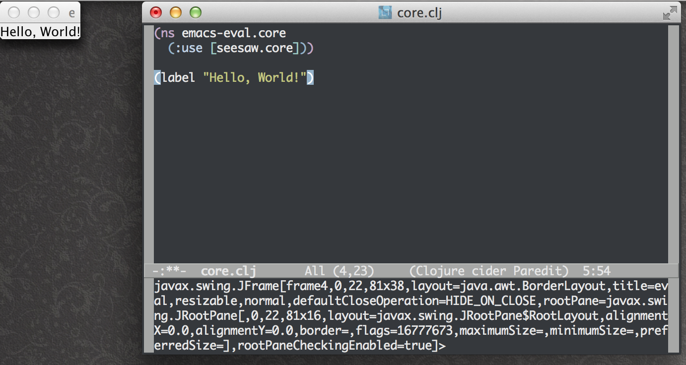
If you have to use Swing, your pain can be slightly mitigated by having a quick way to view components. This will give you a shortcut to pop up a new frame that contains what your expression evaluates to:
This plays nicely with Seesaw, but doesn’t presume that you have it on your classpath. Here’s what it looks like when you C-c f at the end of an expression that defines a Swing component:
Benchmarking with Criterium
In A Few Interesing Clojure Microbenchmarks, I mentioned Hugo Duncan’s Criterium library. It’s a reliable way of measuring the performance of an expression. We can bring it closer to our fingertips by making a function for benchmarking an expression instead of just evaluating it:
I find this simple pattern to be quite handy. Also, when I’m showing off the power of nrepl to the uninitiated, being able to invoke arbitrary functions on whatever is at my cursor looks like pure magic.
I hope you find this useful and if you invent any useful bindings or alternative ways of implementing this pattern, please share!
]]><![CDATA[java.awt.Shape's Insidious Insideness]]>2014-04-30T11:41:00-07:00http://adereth.github.io/blog/2014/04/30/java-dot-awt-dot-shapes-insidious-insidenessI recently added text support to the scad-clj 3D modeling library and encountered an interesting bug:
See that 4? No hole! Why?!? All the other holes are there…
Shape Outlines
First, let’s look at how you get the outline of some text in a font in Java:
We end up with a PathIterator that traces along the outline of the character. This code uses the version of getPathIterator that specifies “flatness”, which means that we get back a path strictly made up of straight line segments that approximate the curves.
Characters that are made from a single filled polygon are relatively easy; there is a single path and the bounded area is what gets filled:
The complexity comes when the path crosses over itself or if it is discontinuous and contains multiple outlines:
The JavaDocs for PathIterator explain a bit about how to actually determine what is inside the path. All of the fill areas are determined using the WIND_EVEN_ODD rule: a point is in the fill area if it is contained by an odd number of paths.
For example, the dotted zero is made up of three paths:
The outline of the outside of the oval
The outline of the inside of the oval
The outline of the dot
The points inside #1 but outside #2 are in 1 area and the points inside #3 are inside 3 areas.
Counting Areas
For each path, we need to count how many other paths contain it. One way is to use java.awt.geom.Path2D.Double to make a Shape and then use the contains(double x, double y) method to see if any of the points from the other paths are in it.
I incorrectly assumed that each Shape contained at least one of the points that define it’s outline. It usually does, which is why all the other holes were properly rendered, but it doesn’t for some shapes, including triangles in certain orientations!
The JavaDoc for Shape says that a point is considered to lie inside a Shape if and only if:
It lies completely inside the Shape boundary or
It lies exactly on the Shape boundary and the space immediately adjacent to the point in the increasing X direction is entirely inside the boundary or
It lies exactly on a horizontal boundary segment and the space immediately adjacent to the point in the increasing Y direction is inside the boundary.
The three points defining the triangle that form the hole in 4 don’t meet any of these criteria, so instead of counting as being in 2 paths (itself and the outer outline), it was counted as being in 1. The fix was to explicitly define a path as containing itself.
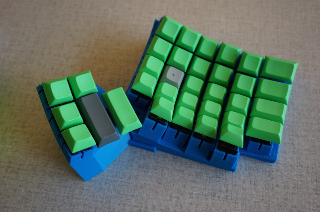
]]><![CDATA[3D Printing with Clojure]]>2014-04-09T07:02:00-07:00http://adereth.github.io/blog/2014/04/09/3d-printing-with-clojureI’ve been doing some 3D printing for my next keyboard project and I’ve got a workflow that I’m pretty happy with that I’d like to share.
When I first started trying to make models a month ago, I tried Blender. It’s an amazing beast, but after a few hours of tutorials it was clear that it would take a while to get proficient with it. Also, it is really designed for interactive modeling and I need something that I can programmatically tweak.
OpenSCAD
A couple of friends suggested OpenSCAD, which is touted as “the programmers’ solid 3D CAD modeler.” It provides a power set of primitive shapes and operations, but the language itself leaves a bit to be desired. This isn’t a beat-up-on-SCAD post, but a few of the things that irked me were:
Strange function application syntax (parameters in parens after the function name with an expression or block following the closing paren)
Unclear variable binding rules (multiple passes are made over the code and the results of changing a variable may affect things earlier in the code unexpectedly)
No package/namespace management
Multiple looping constructs that depend on what you are going to do with the results, not on how you want to loop
scad-clj
Fortunately, Matt Farrell has written scad-clj, an OpenSCAD DSL in Clojure. It addresses every issue I had with OpenSCAD and lends itself to a really nice workflow with the Clojure REPL.
To get started using it, add the dependency on [scad-clj "0.1.0"] to your project.clj and fire up your REPL.
All of the functions for creating 3D models live in the scad-clj.model namespace. There’s no documentation yet, so in the beginning you’ll have to look at the source for model.clj and occassionally the OpenSCAD documentation. Fortunately, there really isn’t much to learn and it’s quite a revelation to discover that almost everything you’ll want to do can be done with a handful of functions.
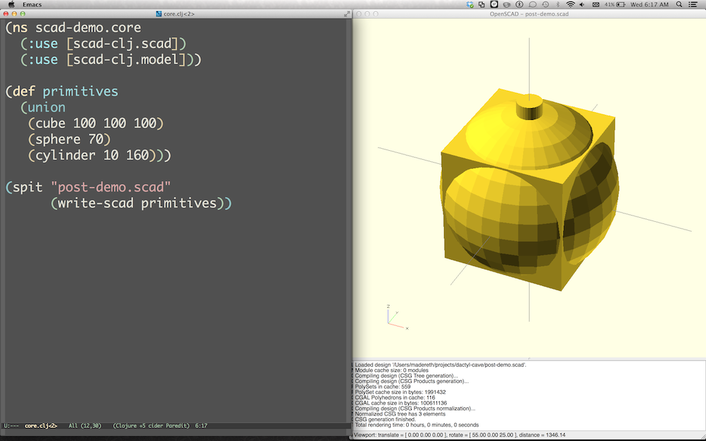
Here’s a simple model that showcases each of the primitive shapes:
Evaluating this gives us a data structure that can be converted into an .scad file using scad-clj.scad/write-scad to generate a string and spit.
12
(spit"post-demo.scad"(write-scadprimitives))
We’re going to use OpenSCAD to view the results. One feature of OpenSCAD that is super useful for this workflow is that it watches opened files and automatically refreshes the rendering when the file is updated. This means that we can just re-evaluate our Clojure code and see the results immediately in another window:
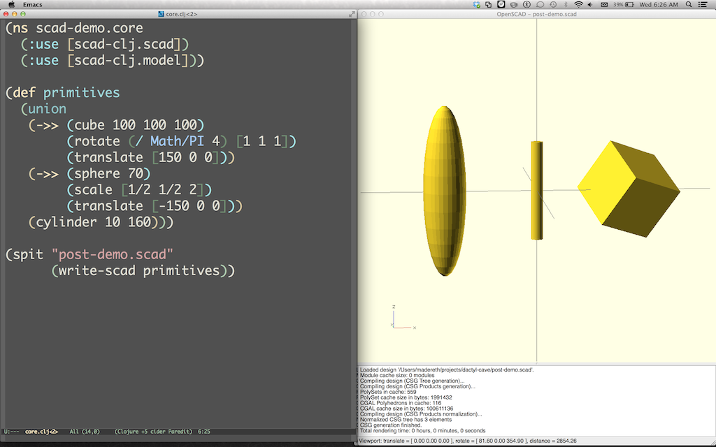
scad-clj makes all new primitive shapes centered at the origin. We can use the shape operator functions to move them around and deform them:
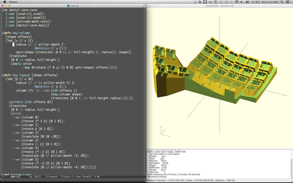
I snuck union into those examples. Shapes can also be combined using intersection, difference, and hull. It’s pretty incredible how much can be done with just these. For example, here’s the latest iteration of my keyboard design built using clj-scad:
3D Printing
Once your design is complete, you can use OpenSCAD to export it as an STL file which can then be imported to software like ReplicatorG or Makerware for processing into an .x3g file that can be printed:
]]><![CDATA[Finishing up the ErgoDox]]>2014-02-27T22:43:00-08:00http://adereth.github.io/blog/2014/02/27/finishing-up-the-ergodoxI’ve been busy with a few other keyboard projects since my last post on my ErgoDox build. While working on those projects, I’ve gotten some parts and done a few more tweaks to the ErgoDox that I’d like to share.
PBT DSA Keycaps
The biggest improvement was switching the keycaps. Originally I had used keycaps from WASD Keyboards that were designed to be used with a normal keyboard. Typical keyboards use keycaps that are very similar to DCS profile caps, which have different profiles for different rows:
In contrast, DSA keycaps have concave spherical tops and are uniform in profile:
I had ordered a set of DSA keycaps from Signature Plastics for another project and decided to try them out on the ErgoDox:
I was surprised with how much better these felt, particularly on the thumb cluster. I now realize that a lot of my discomfort reaching the upper keys on the the thumb cluster came from their relatively high profile.
The DSA keycaps are also made out of PBT plastic instead of ABS. They have a nice textured feel and the plastic is supposed to be much more robust. As I said in my last post, Pimp My Keyboard shop has PBT DCA blank sets for the ErgoDox for $43, which is a great deal and is definitely the way to go if you’re sourcing your own parts.
TRRS Connector
DigiKey finally got the TRRS connectors in stock and sent them to me. I was concerned that they wouldn’t fit in my lower profile case, but a little Dremel action made it work:
The keyboard didn’t work after I added the connector. It worked fine if I just had the right side plugged in, but as soon as I connected the left side, neither worked. I took the whole thing apart and used an ohmmeter to test the 4 connections between the two halves. It turned out that all of the connections were there, but there was a little resistance on one of them. I resoldered it more thoroughly and everything worked fine.
Sanding
Finally, I did a little experimentation with wet sanding the sides to remove some of the burn marks from the paper during the laser cutting and to give a more even finish. I used 400 grit sandpaper and made a little progress:
Acrylic dust is nasty stuff! It didn’t make as much of a difference as I hoped. I’m going to do a little more experimentation sanding with acetone to see if I can melt it smoothly and make the 5 layers of acrylic look like one piece.
Next Steps
My next project is going to involve a lot of acrylic bending, so I’m probably going to also take a stab at cutting and bending a stand for the ErgoDox that tents it at a better angle. Any suggestions are appreciated!
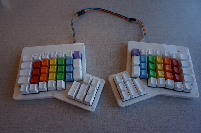
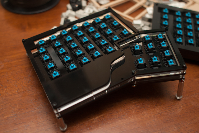
]]><![CDATA[Sourcing and Building an ErgoDox Keyboard]]>2014-02-12T07:25:00-08:00http://adereth.github.io/blog/2014/02/12/building-an-ergodoxThe ErgoDox is a split ergonomic keyboard project. One of the most notable things about it is that you can’t buy this keyboard — you have to build it yourself! The parts list is available on the site, along with the designs for the PCB and case.
I recently built one, sourcing the parts myself, and I’d like to share what I’ve learned.
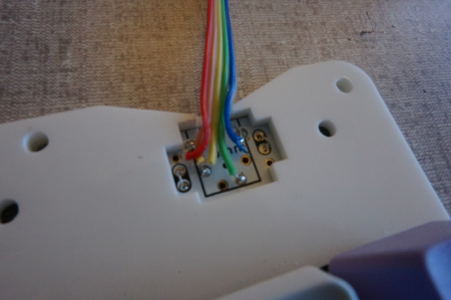
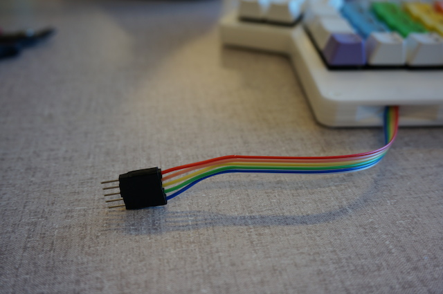
I managed to pick up all the little electronic components from DigiKey, except for the TRRS connectors which are currently unavailable. The TRRS connectors are the headphone-style jacks that are used to connect the two halves. I decided to not use TRRS and to just solder basic wires directly onto the board.
The PCBs were \$38, the keyswitches were \$49, the Teensy was \$22 (but can be bought for less), and the rest of the components came out to about \$20. This \$129 covers everything needed except for the case and the keycaps. For reference, the Massdrop group buy is \$199 for everything excluding the keycaps, so I had roughly $70 to spend on the case before it would have made financial sense to wait for another group buy opportunity.
Making the Case
There are really two options for making a case:
3-D printing
Laser cut acrylic
The designs for the case are available on Shapeways, but it comes out to almost \$200, even when choosing the least expensive options for everything! I considered printing it myself on the Makerbots at my office, but I was skeptical that the older models we have would result in acceptable quality.
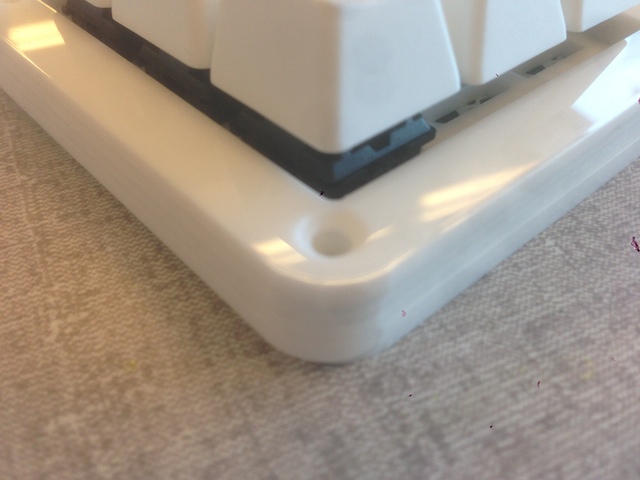
Laser cutting the acrylic seemed like the way to go, so I picked up 5 12”x12” sheets of 3mm opaque white acrylic from Canal Plastics for \$7 a sheet. They can be ordered from Amazon for basically the same price. The design used in Massdrop’s kit uses 3mm sheets for the top and bottom and 5mm sheets for the middle 3 layers, but I believed (hoped!) that I could make it all fit in a slimmer case.
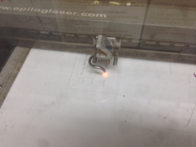
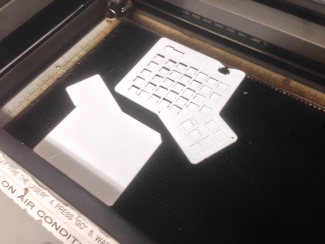
I had never laser cut anything before, but my coworker Trammell has a ton of experience with it and helped me out. He’s a member at NYC Resistor and they have a laser! We used Inkscape to generate PDFs and then used his command line laser cutting tool to send them over to the Epilog laser cutter. We were able to get 2 layers out of each sheet, as you can see in these action shots:
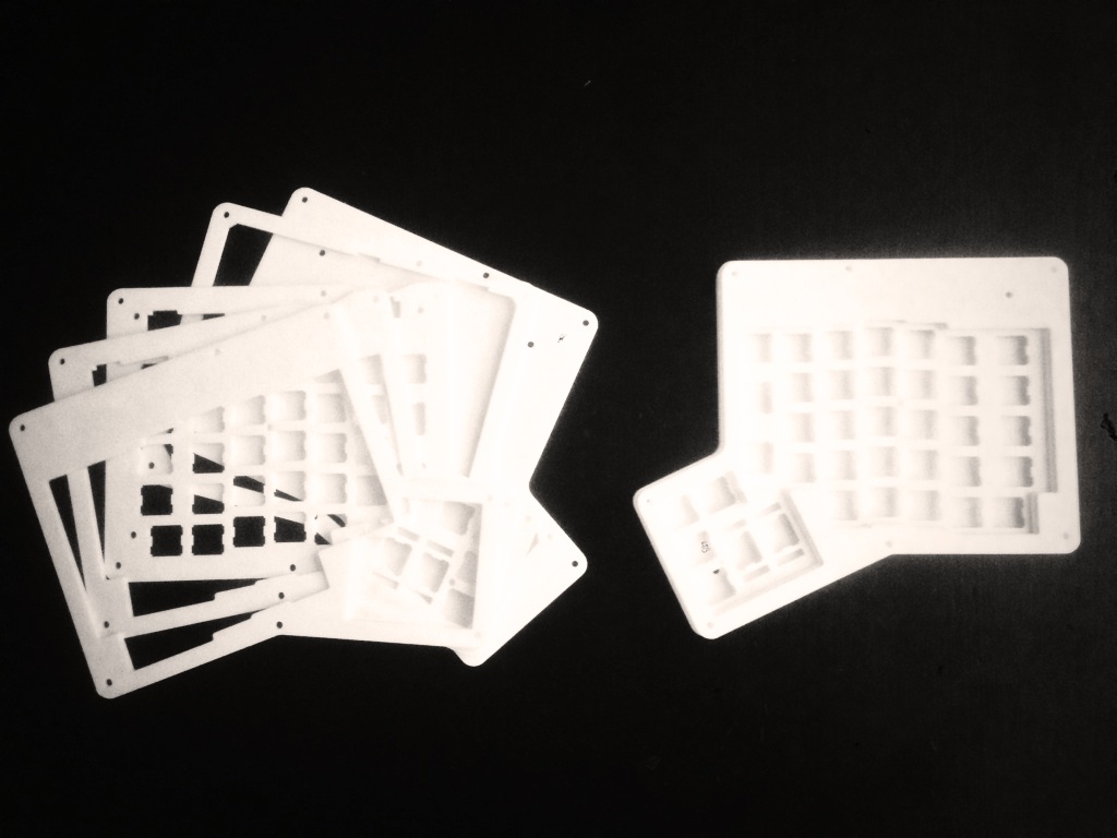
And the final result:
It took just under 27 minutes of actual laser time, which at \$0.75/min came out to \$20. \$55 for the case was a lot more than I expected, but it still kept the cost below \$199. It seems like this is the part that would offer the most savings if done as part of a group buy.
Keycaps
Massdrop usually offers a separate group buy of PBT DCS keycaps when they offer the full kit. I decided to try using standard keycaps and to buy the missing ones separately. This was a big mistake. A proper set of keycaps for the ErgoDox requires 12 1.5x keycaps, which are way too expensive when bought separately. Only later did I discover that the Pimp My Keyboard shop has PBT DCA blank sets for the ErgoDox for $43.
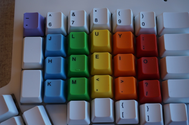
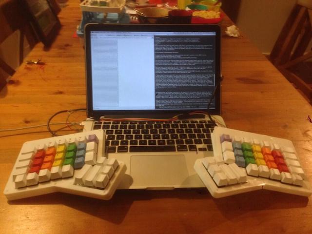
I got my keycaps from WASD Keyboards. They have a pretty slick keycap designer. I used it with my kids and we came up with a design they were happy with (my 3 year-old is currently obsessed with rainbows):
I decided to take advantage of their ability to print whichever letters I want on each key to make this be the Colemak layout. I’ve got the layout commited to muscle memory, but sometimes my kids want to type on my keyboard and it’s annoying to switch to QWERTY so the keys match the letters printed on them.
Putting It Together
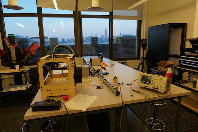
I did the actual soldering and assembly in the Hackerlab at my office:
To put it together, I mostly followed Massdrop’s assembly instructions. I did a decent job soldering (it’s almost 400 solder points), but I wish that I had watched the EEVblog videos on soldering beforehand. That guy knows what he’s talking about.
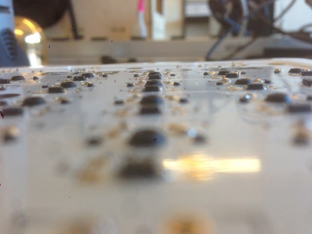
Because I used 3mm sheets instead of the recommended 5mm, there wasn’t a lot of clearance and I had to get creative. The keyswitches stuck out a little too far on the bottom of the PCBs, so I used flush cutters to trim the leads and the plastic nubs:
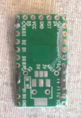
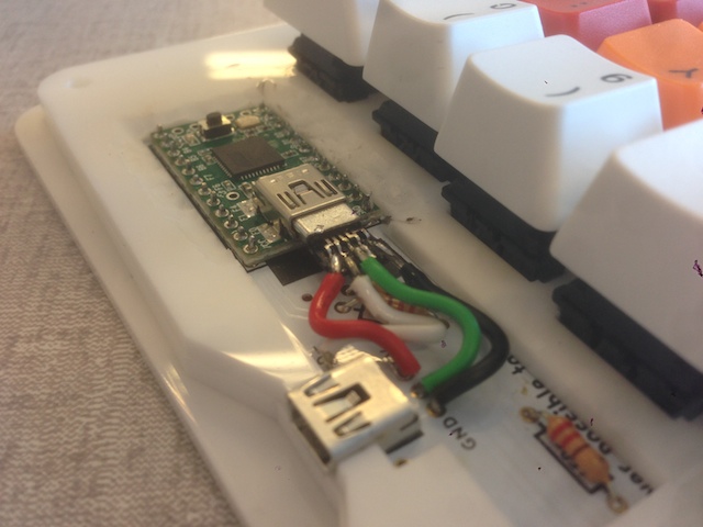
Originally, I used the recommended header pins to connect the Teensy to the PCB, but that brought the USB connector too high and prevented the top layer from fitting. Instead, Trammell suggested I mount it directly on the PCB. Desoldering the Teensy was really, really hard. The throughholes are tiny and there are so many of them! I ended up using the Dremel to clear some space around it and then used the cutting wheel to slice the header pins. Unfortunately, I got the angle wrong one time and took out a nice chunk of the Teensy’s bottom:
I got a replacement Teensy. With some electrical tape on the bottom, I put it directly on the PCB which got me the clearance I needed:
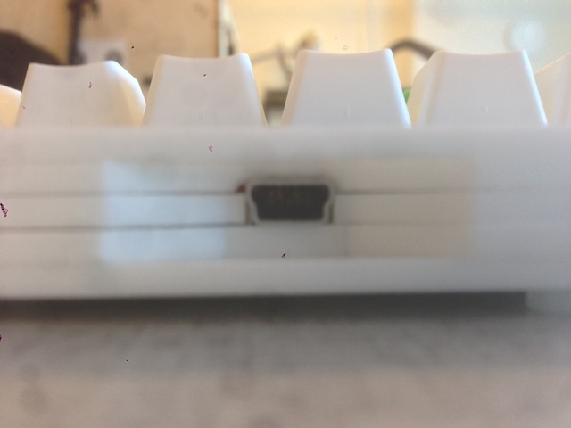
The mini-USB port on the back is about 5mm tall, so it also prevented the layers from fitting together nicely. I remedied that by dremeling a little into the 4th layer. It’s not beautiful, but it’s in the back and it’s good enough.
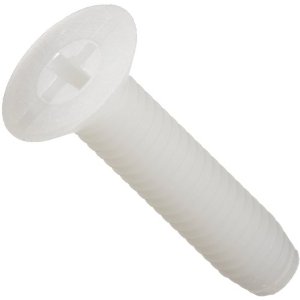
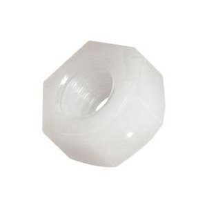
The Massdrop kit includes metal screws and nuts that are seriously sharp and will gouge the surface you put the ErgoDox on:
The Dremel came in handy again for making countersinks and for shortening the screws:
The only other deviation from the original design was that I didn’t use the audio jack style connector. This was motivated by the fact that Digikey didn’t have it in stock and that the jack would be too tall for the 3mm sheets. I just soldered the wires directly onto the PCB:
Programming the Teensy
I used the most excellent ErgoDox Layout Configurator provided by Massdrop to make my own modified layout that matches what I use on my Kinesis Advantage. It was pretty straightforward. I made one of the inner 1.5x keys switch to a QWERTY layer as a courtesy to anyone else who wants to try it out.
Final Product
Here’s how it came out:
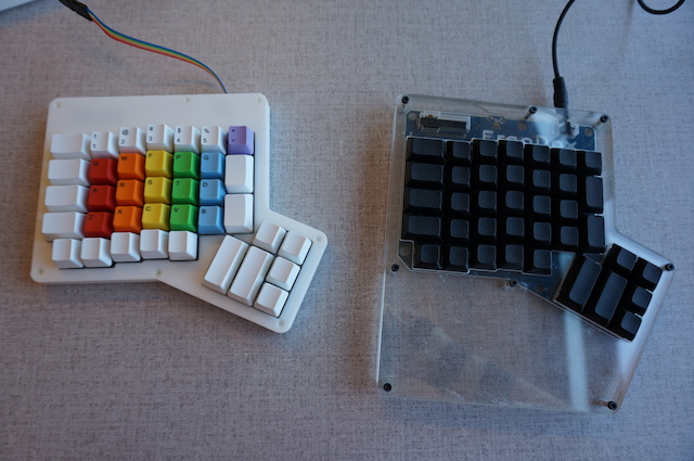
Side-by-side comparison with one of my coworkers’ build of Massdrop’s kit with the palm rest:
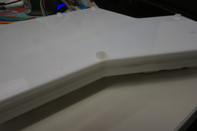
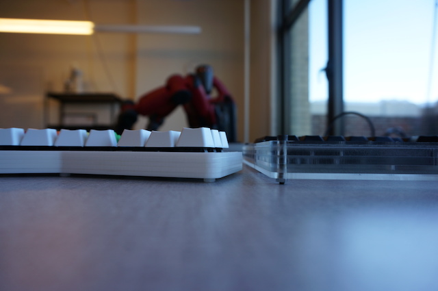
And here you can see just how much thinner the case is with all 3mm sheets:
The keycaps I used were taller than the PBT DCS ones sold by Massdrop, so it ended up being close to the same height.
Review and Next Steps
The design and build were fun, but the real test is actually typing on it. Like the Kinesis Advantage and Truly Ergonomic, the ErgoDox features a columnar layout with staggered keys, which is much more comfortable for me than the traditional layout. Unfortunately, the PCB is flat and I find it to be less comfortable than the Kinesis’s bowl shape. It’s hard to manufacture curved or flexible PCBs, so it’s understandable that this DIY project wouldn’t require it.
A common complaint about the ErgoDox is that the thumb clusters are too close to the other keys. This turned out to be a real problem for me as it requires a serious contortion for me to his the top keys of the thumb cluster. On the Kinesis, I have these mapped to the oft used Ctrl and Alt keys. It was so bad that I ended up having to remap the bottom corner keys to Ctrl and Alt and relegate the top 2 keys to less used ones. I’m not the only one who has struggled with this and the best solution I’ve seen so far is AcidFire’s Grand Piano design:
Another issue is that I chose the wrong keyswitches. My primary keyboard is the Kinesis Advantage LF, which uses Cherry MX reds. I love them, but they are really hard to find at a reasonable price. I wasn’t about to spend $160 on the keyswitches, so I opted for Cherry MX blacks. They are linear feel like the reds, but much stiffer, with an activation force of 60cN instead of 45cN. This didn’t seem like a big deal when I tried it out with individual switches from a sampler set, but it was a whole other experience when trying to type on a full set. It’s much harder to type on and I could feel my fingers straining very quickly.
The last issue is that the ErgoDox really need to be tented at an angle for maximum comfort. My plan was to use this as an ergonomic solution while traveling and I have some designs that would make it easy to attach to my laptop in a tented position. Something like this:
I decided to hold off on this until I have a solution for the other issues I listed.
Conclusion
Overall, this was an incredibly fun project and I learned a ton about how keyboards are made. For anyone who’s waiting for the next Massdrop group buy of a kit, you should know that it can be done by yourself for about the same price if you can get access to a laser cutter or CNC mill to make the case. I’m sure someone can be more creative and come up with an even more accessible solution.
Unfortunately, I’m not thrilled with the actual typing experience, so I can’t recommend it over the Kinesis Advantage. Some people love it, so try it out for yourself if you can or at least print out a stencil of it before committing.
My plan is to take what I’ve learned and to try and build something that’s an even better fit for my travel usage. Hopefully I can procure some Cherry reds for a reasonable price in the future…
]]><![CDATA[Where LISP Fits]]>2014-02-03T07:19:00-08:00http://adereth.github.io/blog/2014/02/03/where-lisp-fitsThere are a lot of great essays about the power and joy of LISP. I had read a bunch of them, but none convinced me to actually put the energy in to make it over those parentheses-shaped speed bumps. A part of me always wanted to, mostly because I’m convinced that our inevitable robot overlords will have to be programs that write programs and everything I had heard made me think that this would likely be done in a LISP. It just makes sense to be prepared.
Almost two years ago, a coworker showed me some gorgeous code that used Clojure’s thrush macro and I fell in love. I found myself jonesing for C-x C-e whenever I tried going back to Java. I devoured Programming Clojure, then The Joy of Clojure. In search of a purer hit, I turned to the source: McCarthy’s original paper on LISP. After reading it, I realized what someone could have told me that would have convinced me to invest the time 12 years earlier.
There’s a lot of interesting stuff in that paper, but what really struck me was that it felt like it fit into a theoretical framework that I thought I already knew reasonably well. This post isn’t about the power of LISP, which has been covered by others better than I could. Rather, it’s about where LISP fits in the world of computation.
None of what I’m about to say is novel or rigorous. I’m pretty sure that all the novel and rigorous stuff around this topic is 50 – 75 years old, but I just wasn’t exposed to it as directly as I’m going to try and lay out.
One aspect that I really enjoyed was that there was a narrative; we started with Finite State Automata (FSA), analyzed the additional power of Pushdown Automata (PDA), and saw it culminate in Turing Machines (TM). Each of these models look very similar and have a natural connection: they are each just state machines with different types of external memory.
The tape in the Turing Machine can be viewed as two stacks, with one stack representing everything to the left of the current position and the other stack as the current position and everything to the right. With this model, we can view the computational hierarchy (FSA –> PDA –> TM) as just state machines with 0, 1, or 2 stacks. I think it’s quite an elegant representation and it makes the progression seem quite natural.
A key insight along the journey is that these machines are equivalent in power to other useful systems. A sizable section in the chapter on Finite State Automata is dedicated to their equivalence with Regular Expressions (RegEx). Context Free Grammars (CFG) are actually introduced before Pushdown Automata. But when we get to Turing Machines, there’s nothing but a couple paragraphs in a section called “Equivalence with Other Models”, which says:
Many [languages], such as Pascal and LISP, look quite different from one another in style and structure. Can some algorithm be programmed in one of them and not the others? Of course not — we can compile LISP into Pascal and Pascal into LISP, which means that the two languages describe exactly the same class of algorithms. So do all other reasonable programming languages.
The book and class leave it at that and proceed onto the limits of computability, which is the real point of the material. But there’s a natural question that isn’t presented in the book and which I never thought to ask:
While we know that there are many models that equal Turing Machines, we could also construct other models that equal FSAs or PDAs. Why are RegExs and CFGs used as the parallel models of computation? With the machine model, we were able to just add a stack to move up at each level – is there a natural connection between RegExs and CFGs that we extrapolate to find their next level that is Turing equivalent?
The left-hand side of the relations above are the automaton-based models and the right-hand side are the language-based models. The language models are all implemented as production rules, where some symbols are converted to other symbols. The different levels of computation just have different restrictions on what kind of replacements rules are allowed.
For instance RegExs are all rules of the form $A \to a$ and $A \to aB$, where the uppercase letters are non-terminal symbols and the lowercase are terminal. In CFGs, some of the restrictions on the right-hand side are lifted. Allowing terminals to appear on the left-hand side lets us make rules that are conditional on what has already been replaced, which appropriately gets called “Context Sensitive Grammars.” Finally, when all the rules are lifted, we get Recursively Enumerable languages, which are Turing equivalent. The Wikipedia page for the hierarchy and the respective levels is a good source for learning more.
When you look at the definition of LISP in McCarthy’s paper, it’s much closer to being an applied version of Chomsky’s style than Turing’s. This isn’t surprising, given that they were contemporaries at MIT. In McCarthy’s History of Lisp, he expicitly states that making a usable version of this other side was his goal:
These simplifications made LISP into a way of describing computable functions much neater than the Turing machines or the general recursive definitions used in recursive function theory. The fact that Turing machines constitute an awkward programming language doesn’t much bother recursive function theorists, because they almost never have any reason to write particular recursive definitions, since the theory concerns recursive functions in general. They often have reason to prove that recursive functions with specific properties exist, but this can be done by an informal argument without having to write them down explicitly. In the early days of computing, some people developed programming languages based on Turing machines; perhaps it seemed more scientific. Anyway, I decided to write a paper describing LISP both as a programming language and as a formalism for doing recursive function theory.
Here we have it straight from the source. McCarthy was trying to capture the power of recursive definitions in a usable form. Just like the automata theorists, once the linguists theorist hit Turing completeness, they focused on the limits instead of the usage.
Theoreticians are more interested in the equality of the systems than the usability, but as practitioners we know that it matters that some problems are more readily solvable in different representations. Sometimes it’s more appropriate to use a RegEx and sometimes an FSA is better suited, even though you could apply either. While nobody is busting out the Turing Machine to tackle real-world problems, some of our languages are more influenced by one side or the other.
Turing Machines Considered Harmful
If you track back the imperative/functional divide to Turing Machines and Chomsky’s forms, some of the roots are showing. Turing Machines are conducive to a couple things that are considered harmful in larger systems: GOTO-based1 and mutation-centric2 thinking. In a lot of cases, we’re finding that the languages influenced by the language-side are better suited for our problems. Paul Graham argues that the popular languages have been steadily evolving towards the LISPy side.
Anyway, this is a connection that I wish I had been shown at the peak of my interest in automata theory because it would have gotten me a lot more excited about LISP sooner. I think it’s interesting to look at LISP as something that has the same theoretical underpinnings as these other tools (RegEx and CFG) that we already acknowledged as vital.
]]><![CDATA[Every project.clj]]>2014-01-20T17:33:00-08:00http://adereth.github.io/blog/2014/01/20/every-project-dot-cljI was recently looking for an interesting relational dataset for another project and the idea of using the dependencies for every Clojure project on GitHub came up. It turns out that it’s possible to download almost every project.clj using Tentacles, so I decided to…
The most annoying part was dealing with GitHub’s rate limits, but after waiting a few hours I had them all on local disk and was able to play around. I haven’t gotten to dig into the data for the actual project I’m doing, but there were a couple simple queries that I thought were worth sharing.
Most frequently included packages
I was able to download 10770 project.clj files. Here are the 50 most frequently included packages listed in their :dependencies:
Dependency
Count
org.clojure/clojure-contrib
1524
compojure
1348
hiccup
743
clj-http
738
ring/ring-jetty-adapter
607
cheshire
558
org.clojure/data.json
552
clj-time
526
org.clojure/tools.logging
490
enlive
444
noir
388
ring/ring-core
375
ring
361
org.clojure/tools.cli
348
org.clojure/java.jdbc
344
org.clojure/clojurescript
339
org.clojure/core.async
235
midje
227
org.clojure/math.numeric-tower
219
korma
206
incanter
202
seesaw
195
overtone
172
slingshot
160
quil
158
com.taoensso/timbre
150
http-kit
149
ring/ring-devel
145
org.clojure/math.combinatorics
145
org.clojure/core.logic
138
environ
132
aleph
132
log4j
131
ch.qos.logback/logback-classic
125
org.clojure/tools.nrepl
124
congomongo
124
com.datomic/datomic-free
123
com.novemberain/monger
123
lib-noir
121
org.clojure/core.match
118
ring/ring-json
111
clojure
110
org.clojure/data.xml
110
log4j/log4j
109
mysql/mysql-connector-java
109
postgresql/postgresql
107
org.clojure/data.csv
101
org.clojure/tools.trace
98
org.clojure/tools.namespace
92
ring-server
92
I think it makes a nice hit-list of projects to check out!
A couple interesting things jumped out at me:
12.5% of Clojure projects on GitHub are using Compojure. Impressive.
congomongo, com.novemberain/monger, com.datomic/datomic-free, mysql/mysql-connector-java, and postgresql/postgresql are all clustered together in the low 100’s.
Most frequently applied licenses
Just over half of the project.clj’s don’t contain a :license. Here are the most popular:
License
Count
EPL
4430
MIT
336
Apache
106
BSD
92
GPL
90
LGPL
25
CC
21
WTFPL
18
AGPL
11
Mozilla
11
The EPL’s dominance doesn’t come as a surprise, given Clojure’s use of it for the core libraries.
23 projects have “WTF” or “fuck” in their license string:
License
Count
WTFPL
18
Do What The Fuck You Want To Public License
3
DO WHAT THE FUCK YOU WANT TO PUBLIC LICENSE Version 2
1
All Rights Reserved Muthafucka
1
Conclusion
I’d like to share a mirror of just the project.clj files wrapped up in a single download, but I want to be conscientious of the variety of licenses. I’ll clean up the code for pulling and summarizing all this data soon so others can play with it. In the meantime, feel free to suggest other analyses that could be done on these…
]]><![CDATA[Quine Tweet Challenge]]>2014-01-08T07:49:00-08:00http://adereth.github.io/blog/2014/01/08/quine-tweet-challengeA quine is a program which takes no input and outputs a copy of its own source code. There’s a history of making challenges out of variants on the idea (shortest quine, Ouroboros Programs, Multiquines). I’d like to propose a new variant for our modern social age: the Quine Tweet.
Seeing him tweet source code that tweets got me thinking about code that tweets its own source code. Could a Quine Tweet be written? I took a stab at adapting my Clojure code for Gus’s Quinundrum, but I just couldn’t make it fit in 140 characters.
If you paste it into a notebook and evaluate, you’ll get prompted for authorization and it’ll post itself. Here’s a brief explanation of what it does:
$Line is the count of input expressions that have been evaluated.
InString is a function that gets the input for the ith input expression. It returns a string that has some extra escaped parentheses.
92 is the ASCII code for \\. 40 and 41 are the codes for ( and ). FromCharacterCode can take a list of lists of ASCII codes and return a list of strings. The list is destructured into the variables o (open) and c (close).
StringReplace is then used to clean up the extra parentheses.
SendMessage is the new function in the Wolfram language that does all the hard work of posting.
I don’t think this is really in the true spirit of a quine, as having something like InString makes it a bit trivial, but you do what you must when you only have 140 characters!
The Challenge
So, can it be done in any other languages? Here’s what I think are fair restrictions:
Any standard Twitter client library for your language can be linked using the language’s normal methods (pom.xml, project.clj, etc.)
The authorization token can be supplied outside of source, either interactively or through a text file. I don’t imagine anyone wants to be sharing that…
Bonus points if you manage to make the tweet and source include #quine!
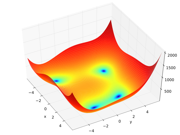 Himmelblau’s Function, a popular test function for black-box optimization


