For the past year, I’ve been completely obsessed with Apex Legends, a battle royale game that pits 20 teams of 3 players against each other in a shrinking map. Teams fight and eliminate each other until a single team is left standing.

I’ve watched my win rate for each competitive season of the game and wondered what a reasonable win rate for an average player might be. There are a bunch of factors to consider and the more I thought about the more I realized I’d need to turn to simulation understand how the factors would interact with each other. I’m going to share my thinking and results and I’d love to hear what else should be considered.

Initial Expectations

In a simple world where all players are of equal skill, you’d expect the win rate for all players to converge to 0.05, since there are 20 teams in each match.

Not all players are equal, of course! We might expect that an average-skilled player will have a win rate significantly below 0.05, since you have to beat everyone and it’s very likely there will be better players present in each match.

Since it’s an elimation style game, worse players will return to the queue of players for the next game at a much faster rate than better players. We would then expect to see the distribution of players in each game to not be the same as the overall population distribution. Worse players will be overrepresented in each game, possibly driving the win rate for average-skilled players up.

Another important consideration is that it’s a team game and the teams are totally random if we assume everyone is solo-queueing. This could have an averaging effect on each team’s aggregate skill, pushing the expected win rate closer to 0.05. We’ll also see that the choice of aggregation function will have a big impact on the expected win rate of best and worst players.

We have some factors that could push the expected win rate for an average-skilled player over 0.05, under 0.05, and towards 0.05. How do these factors interact? Which matter most?

Basic Simulation Framework

We’ll simulate the behavior of an entire population by maintaining two queues. One is a queue of players waiting to join a new game and the other is a queue of active games from which players will be eliminated and returned to the waiting queue.

Start by populating the waiting queue with a set of players with skills sampled from a distribution. Then, in a loop:

1. Check if there are at least gameSize players in the waiting queue to start a new game. We need 60 players for a game in Apex Legends.
2. If there are, randomly assign the players to teams of size teamSize.
3. Apply a teamSkillFunction to each team to compute the aggregated team skill.
4. Apply a probabilistic sort using the team skills as weights to determine the order in which teams will be elimated.
5. Add the newly created game to the end of the active game queue.
6. Move the next eliminated team from the head of the active game queue to the waiting queue.
7. If there are any teams remaining in the active game selected in step #6, put the updated game at the end of the active game queue.

Probabilistic Sorting

One design decision is how to determine the results of a game given a set of skill values for each team. The approach I took was to treat the skill value as a weight and to sample from the weighted discrete distribution to pick a winner. We continue to pick a team from the remaining teams until a full elimation order has been chosen.

This ordering can be computed by doing random selection as described above, but it can also be done efficiently by sampling a value for each team $i$ from a beta distribution parameterized as $\text{B}(1, w_i)$ and then sorting by the sampled values. This ends up giving the same result because $$P(x < y \mid x \sim \text{B}(1, w_i), y \sim \text{B}(1, w_j)) = \frac{w_i}{w_i + w_j}$$ …which I think is a pretty neat result.

Mathematica’s built-in RandomSample function was used to compute these weighted pseudorandom permutations.

This method is a dramatic simplification of how games actually play out, but it’s sufficient for demonstrating a lot of the interesting effects I was hoping to explore.

Simulating a Solo Battle Royale (Tetris 99)

Before we jump into simulating Apex Legends, which has the complexity of figuring out how to combine players skill as a team, let’s look at a simpler battle royale game that has individuals competing:

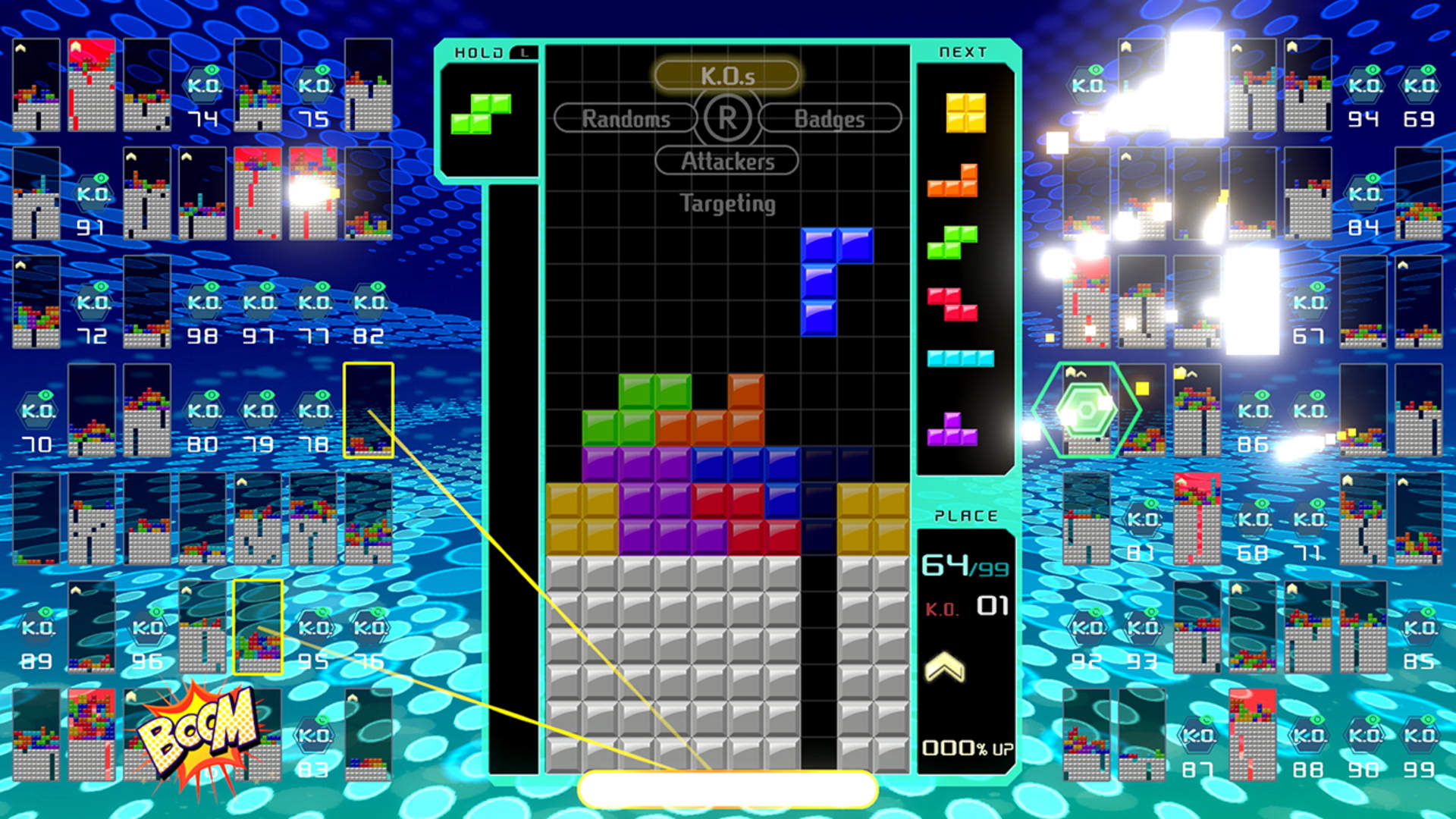
The idea is basically the same and the same simulator defined above can easily be used to explore win rate dynamics here. In Tetris 99, there are 99 players playing Tetris simulatenously. When a player clears multiple lines, they can have junk pieces randomly dropped on any of the other players. Again, the last player standing wins.

Here, we expect the factors that push the expected win rate away from the baseline of 1/99 to be even stronger than in Apex Legends. With 99 players, it’s extremely likely that there will be multiple players better than you, but we also will expect better players to remain in matches much longer and new games will have worse players overrepresented.

First, let’s verify the baseline case by running a simulation where all players have the same skill:

1
2
3
4
5
6
7
8
9
10

tetrisConstantSkill = SimulateBattleRoyale[
   <|
    "playerCount" -> 99,
    "teamSize" -> 1,
    "gameSize" -> 99,
    "iterations" -> 10000000,
    "skillFunction" -> (ConstantArray[1, Length@#] &),
    "teamSkillFunction" -> Total
    |>
   ];

With 1000 players and 10,000,000 iterations, we end up with a normal looking distribution of win rates:

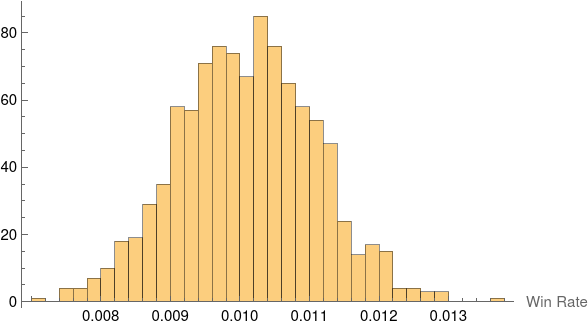
The mean is $0.0101018$, which is very close to $1/99 = 0.\overline{01}$.

Now we can start to explore how the dynamics of differing skills affect the distribution of win rates. Let’s use uniformly distributed player skills. We won’t see the effect of the queue if we have exactly 99 players in our population, so each game contains the full uniformly distributed set of skills.

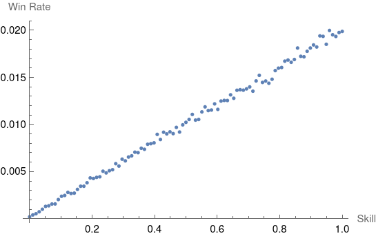
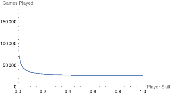
This linear result is expected, since the likelihood of a player $i$ being chosen as the winner is $w_i / \sum_{j=1}^{99} w_j$ and the denominator is a constant. It starts to become interesting and less easy to compute analytically when we introduce the fact that worse players are elimated earlier from the game and returned to the player queue. Let’s run with 1000 players in the population instead of exactly 99:

1
2
3
4
5
6
7
8

tetris = SimulateBattleRoyale[<|
    "playerCount" -> 1000,
    "teamSize" -> 1,
    "gameSize" -> 99,
    "iterations" -> 10000000,
    "skillFunction" -> Identity,
    "teamSkillFunction" -> Total
    |>];

This is where it starts to get interesting! Worse players get elimated earlier, so they queue up for more games and end up with a much higher count of games played:

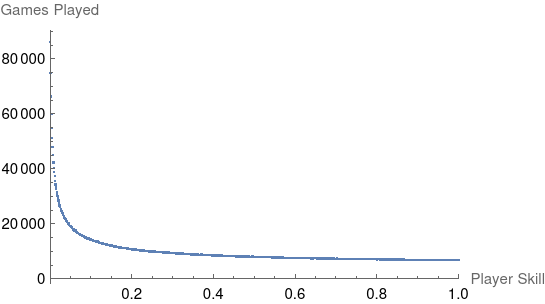
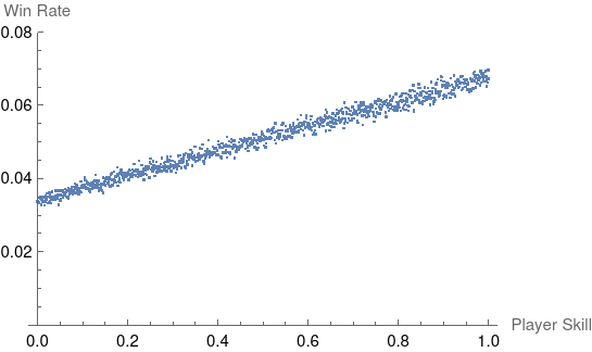
Now that there are 1000 players in the population, the expected win rate for player $i$ is $w_i / \sum_{j=1}^{1000} p_j w_j$, where $p_j$ is the probability that player $j$ is in the game. The plot above is actually the same shape as the PDF of skill levels in an average game and can be used to compute $p$.

We still expect there to be a linear relationship for the win rate, but with a different slope because the denominator is now a different constant. Before the denominator was $\sum_{j=1}^{99} w_j = 99 * ½ = 49.5$, but with the queue dynamics in place and 1000 players, it’s $38.73$. This translates to a $27.8\%$ increase in the expected win rate for each player because they tend to be up against weaker competition.

There are a ton of simplifying assumptions here, but I think the most egregiously wrong is the choice of distribution of for player skill in the population. There’s a long tail of skill, which is supported by my 14.5% win rate:

Created my own account so my filthy casual family stops messing with my Tetris 99 stats pic.twitter.com/PDYxCjPXrL

— Aͫdͣeͭrͭeth (@adereth) March 8, 2019

Simulating Team Games (Apex Legends)

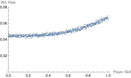
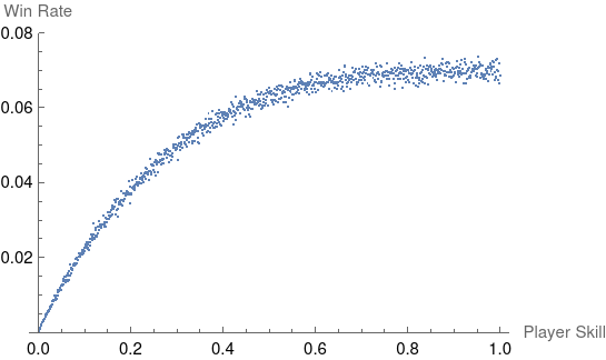
Now that we’ve established that the variable amount of time a player lasts in a game can push up the expected win rate, let’s look at the effect of random 3 person teams. There are a ton of different ways we can choose to aggregate the skill level of a team, but let’s start with the obvious choice of averaging the skills of the team members:

1
2
3
4
5
6
7
8

apexMean = SimulateBattleRoyale[<|
    "playerCount" -> 1000,
    "teamSize" -> 3,
    "gameSize" -> 60,
    "iterations" -> 10000000,
    "skillFunction" -> Identity,
    "teamSkillFunction" -> Mean
    |>];

We still observe an approximately linear win rate but with a key difference: a positive intercept. The expected win rate is now:

$$\frac{w_i/3 + 2 \bar{t} / 3}{w_i/3 + 2 \bar{t} / 3 + 19 \bar{t}}$$

where $\bar{t}$ is the expected average skill level in a game. We’ll assume that the population is large enough that removing player $i$ from the pool of possible players doesn’t significantly affect $\bar{t}$. We can see that in this model even the worst player ($w_i = 0$) has a $\frac{2/3}{19 + 2/3} = 0.0339$ likelihood of winning. It’s interesting to note that the intercept here is independent on the distribution of player skills and only depends on our choice of team aggregation function and winner selection method.

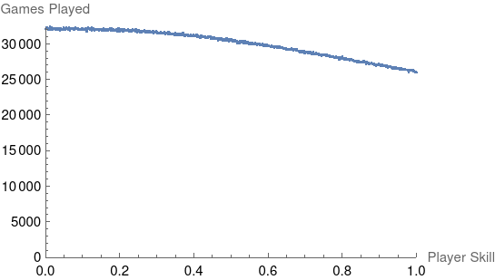
We can also look at the count of games played to get a sense for the expected distribution of player skills in a given game:

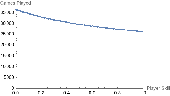
Even though worse players are losing faster and returning to the queue more often, the discrepency between the worst and best players isn’t nearly as dramatic as it was in the Tetris 99 simulation.

Alternative Aggregations

Instead of using the mean of the players, we can experiment with other aggregation functions. We can imagine a game where a teams performance is limited by its worst player by using a min function or a game where strong players are able to carry by using a max function.

Min

1
2
3
4
5
6
7
8

apexMin = SimulateBattleRoyale[<|
    "playerCount" -> 1000,
    "teamSize" -> 3,
    "gameSize" -> 60,
    "iterations" -> 10000000,
    "skillFunction" -> Identity,
    "teamSkillFunction" -> Min
    |>];

This is the first simulation that gives us a win rate plot that doesn’t look linear:

As expected, a player with no chance of winning always loses. It becomes interesting when we look at the win rate of higher skilled players, which starts to flatten around the median since it becomes increasingly likely that there’s a worse player on the team. The benefit of being above average no longer matters in this model.

Max