I’m really excited about Wolfram Research’s announcement that Mathematica and the Wolfram language are now available for free on the Raspberry Pi.

In the announcement, Stephen Wolfram gave this disclaimer:

To be clear, the Raspberry Pi is perhaps 10 to 20 times slower at running the Wolfram Language than a typical current-model laptop (and sometimes even slower when it’s lacking architecture-specific internal libraries).

I’ve got a laptop and a Raspberry Pi, so I decided to put this to the test.

MathematicaMark

Mathematica ships with a benchmarking package called MathematicaMark. The latest version of the benchmark, MathematicaMark9, consists of 15 tests that use both numeric and symbolic functions. The MathematicaMark score is the geometric mean of the reciprocal of the timings, normalized against some reference system’s timings:

$$ \sqrt[15]{\prod_{i=1}^{15} \frac{t_{r,i}}{t_{s,i}}} $$

…where $t_{s,i}$ is the timing for test $i$ on system $s$ and $r$ is the reference system. For MathematicaMark9, the reference system is a 3.07 GHz Core i7-950 with 8 hyper-threaded cores running 64-bit Windows 7 Pro. By definition, this system has a MathematicaMark9 score of 1.0.

We can compare systems using the MathematicaMark score. If a system were 10 to 20 times slower, we would expect its MathematicaMark score to be anywhere from 1/10^th to 1/20^th the value of the faster system. The Benchmark[] function also provides the timings for the individual tests, so we can dig in and see which functions might be benefitting from the architecture-specific internal libraries Wolfram mentioned.

Raspberry Pi Configuration

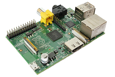
I used a Model B Raspberry Pi with 512MB of RAM. The tests were done after a fresh install of NOOBS 1.3.3, which includes Mathematica and the Wolfram Language installed by default. wolfram was invoked from the commandline and nothing else was running on the system, most notably the X Window System and the Mathematica Notebook interface.

“Typical Current-Model Laptop”

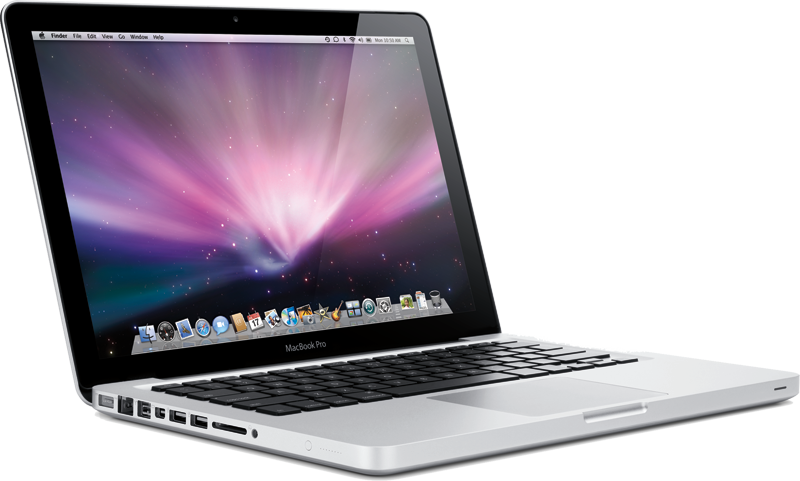
Mathematica ships with benchmark results for 15 different systems (including the reference system). It’s not clear which system to use for this comparison, so I conveniently chose my Early 2013 13-inch Retina MacBook Pro, which sports a 2.6 GHz Intel Core i5 processor (4 hyper-threaded cores) as a representative “typical current-model laptop.” Based on the sea of glowing Apple logos I’ve seen in the audiences of the conferences I attended this year, I think it’s a fair selection.

MathematicaMark9 Scores

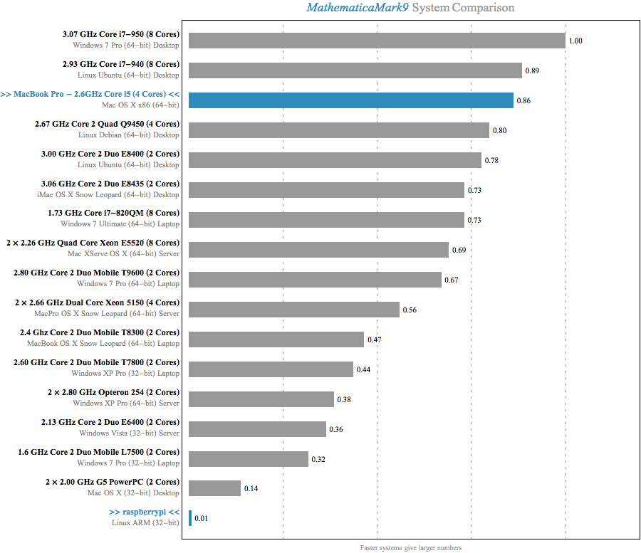
With the setup out of the way, let’s take a look at the report comparing the MacBook, Raspberry Pi, and the 15 included systems:

Click for full-sized report

The MacBook Pro weighs in at a respectible 0.86, while the Raspberry Pi is actually getting rounded up to 0.01 from a true score of 0.005. Running the benchmark takes 16 seconds on the laptop and nearly 49 minutes on the Raspberry Pi.

Even the slowest machine in the included benchmarks score nearly 30x higher. I don’t think Wolfram would consider a pre-Intel Mac to be a “typical current-model” computer. To see the numbers he’s citing, we need to dig into the timings for the individual tests.

Performance on Individual Tests

The source for the 15 individual tests and the timings on a variety of reference systems is included in the full MathematicaMark9 Benchmark Report. Here are the timings on the Raspberry Pi and the Macbook Pro:

Sorting by the ratio reveals that there are definitely cases where the relative performance falls in the 10x – 20x range cited by Wolfram.

It’s interesting to note that the 4 worst performing tests by ratio are all linear algebra operations involving matrix decomposition or multiplication. These are the types of operations that have probably gotten a lot of optimization love from Wolfram Research developers in the past because this is the area that potential users compare when deciding between Mathematica and its competitors, particularly Matlab.

If you look through the revision history highlights of Mathematica, you’ll see that there was a sequence of releases where every version had at least one top-level mention of linear algebra performance improvements:

• Mathematica 5.0 – 2003
  • “Record-breaking speed through processor-optimized numerical linear algebra”
  • “Full support for high-speed sparse linear algebra”
• Mathematica 5.1 – 2004
  • “Numerical linear algebra performance enhancements”
• Mathematica 5.2 – 2005
  • “Multithreaded numerical linear algebra”
  • “Vector-based performance enhancements”

The 5^th worst test by ratio, Elementary Functions, is also interesting to dig into. Here’s the source:

1
2
3
4
5
6
7
8
9
10

Module[{m1, m2},
 Timing[
  SeedRandom[1];
  m1 = RandomReal[{}, {2.2`*^6}];
  m2 = RandomReal[{}, {2.2`*^6}];
  Do[
   Exp[m1];
   Sin[m1];
   ArcTan[m1, m2],
   {30}]]]

It’s computing $ e^x $, $ \sin{x} $, and $ \text{tan}^{-1} \frac{x}{y} $ for lists of 2,200,000 random numbers 30 times. Exp, Sin, and ArcTan all have the Listable attribute, which means that they are automatically mapped over lists that are passed in as arguments. Sin[list] and Map[Sin, list] are functionally equivalent, but the former provides the implementation the opportunity to take an optimized path if there is a faster way of computing the sine of multiple numbers.

We can verify that this is a case where architecture specific optimizations are in play by rewriting the test to use Map and MapThread:

1
2
3
4
5
6
7
8

Module[{m1, m2},
 Timing[
  SeedRandom[1];
  m1 = RandomReal[{}, {2.2`*^6}];
  m2 = RandomReal[{}, {2.2`*^6}];
  Map[Exp, m1];
  Map[Sin, m1];
  MapThread[ArcTan, {m1, m2}];]]

Note that I’m only running this once, as opposed to the 30 times in the original test, because the non-Listable version is so much slower.

The version that doesn’t take advantage of the Listable attribute takes 1.63 seconds on the Macbook Pro and 62.64 seconds on the Raspberry Pi. This ratio of 38.2 (vs. 133.3 before) is much closer to the ratio we see from the other tests that don’t take advantage of specifics of the architecture.

Conclusion

Even though Mathematica is much slower on the Raspberry Pi, it’s a tremendous free gift and it still has many uses:

• A recent guest post from Wolfram Research on the Raspberry Pi blog links to several projects that take advantage of the easy ways of controlling hardware using Mathematica on the Raspberry Pi.

• Much of what most people use Mathematica for doesn’t require extreme performance. For instance, getting the closed form of an integral or derivative is still practically instantaneous from a human’s perspective.

• Just getting to experience the language and environment with only a $35 investment is worthwhile. For developers, there is a lot to learn from the language, which is heavily influenced by Lisp’s M-expressions, and the notebook enviroment, which is just starting to be replicated by iPython. On top of that, the incredible interactive documentation for the language is something everyone should experience.

Any questions, corrections, or suggestions are appreciated!

I’ve been working on a nerd ethnography project with the GitHub API. There’s so much fun data to play with there that it’s inevitable that I’ll get a little distracted…

One distraction was the realization that I could use the search API to get a massive list of the top repos ordered by star count. Once I started looking at the results, I realized that star data is an interesting alternative metric for evaluating language popularity. Instead of looking at which languages people are actually writing new projects using, we can see which languages are used for the most popular projects.

What are stars?

In August 2012, GitHub announced a new version of their notification system that allowed users to easily mark a repository as interesting by “starring” it:

Stars are essentially lightweight bookmarks that are publicly visible. Even though they were introduced just over a year ago, all “watches” were converted to stars so there’s plenty of data.

Which are the most starred repos?

Let’s start by looking at the top 20:

If you want to play with the data yourself, I’ve put a cache of the top 5000 repositories here. I’ve also posted the Clojure code I wrote to collect the data at adereth/counting-stars.

Which languages have the top spots?

In Adam Bard’s Top Github Languages for 2013 (so far), he counted repo creation and found that JavaScript and Ruby were pretty close. The top star counts tell a very different story, with JavaScript dominating 7 of the top 10 spots. CSS was in 11th place in his analysis, but it’s 2 of the top 10 spots.

Observing that 7 of the top 10 spots are JavaScript gives a sense for both the volume and the relative ranking of JavaScript in that range of the leaderboard, but just seeing that another language is 50 of the top 5000 spots doesn’t give nearly as much color.

One approach is to look at the number of repos in different ranges for each language:

The table is interesting, but it still doesn’t give us a good sense for how the middle languages (C#, Scala, Clojure, Go) compare. It also reveals that there are different star distributions within the languages. For instance, CSS makes a showing in the top 10 but it has way fewer representatives (174) in the top 5000 than PHP (248), Objective C (495), or Java (255).

Looking at the top repo for each language also exposes a weakness in the methodology: GitHub’s language identification isn’t perfect and there are number of polyglot projects. The top Java repo is Storm, which uses enough Clojure (20.1% by GitHub’s measure) to make this identification questionable when you take into account Clojure’s conciseness over Java’s.

What about star counts?

Looking at the results after ranking obscures the actual distribution of stars. Using a squarified treemap with star count for the size and no hierarchy is a compact way of visualizing the ranking while exposing details about the absolute popularity of each repo. The squarified treemap algorithm roughly maintains the order going from one corner to the other.

Here are the top 1000 repos, using stars for the size and language for the color:

(Language and repository name shown on mouseover, click to visit repository. A bit of a fail on touch devices right now.)

Despite being a little chaotic, we can start to see some of the details of the distributions. It still suffers from being difficult to glean information about the middling languages. The comparisons become a little easier if we group the boxes by language. That’s pretty easy, since that’s really the intended usage of treemaps.

Here are the top 5000 grouped by language:

Honestly, I’m not really in love with this visualization, but it was a fun experiment. I have some ideas for more effective representations, but I need to work on my d3.js-fu. Hopefully it serves as an inspirational starting point for someone else…

Conclusion

Firstly, GitHub’s API is really cool and can give you some insights that aren’t exposed through their UI. Like I said at the start of this post, I have another project that caused me to look at this API in the first place and I’m really excited for the possibilities with this data.

GitHub’s current UI is really focused on using stars to expose what’s trending and doesn’t really make it easy to see the all-time greatest hits. Perhaps the expectation is that everyone already knows these repos, but I certainly didn’t and I’ve discovered or rediscovered a few gems. My previous post came about because of my discovery of Font Awesome through this investigation.

I’ll close out with a couple questions (with no question marks) for the audience:

1. Through this lens, JavaScript is way more popular than other metrics seem to indicate. One hypothesis is that we all end up exposing things through the browser, so you end up doing something in JavaScript no matter what your language of choice is. I’m interested in other ideas and would also appreciate thoughts on how to validate them.

2. It’s not obvious to me how to best aggregate ranking data. I’d love to see someone else take this data and expose something more interesting. Even if you’re not going to do anything with the data, any ideas are appreciated.

Font Awesome is a gorgeous icon font designed to play nicely with Bootstrap. I was playing around with it today and noticed the highly detailed fa-barcode character:

If we make it a little larger, we can see that it really looks like a legit barcode:

I scanned it with a barcode reader and it’s the code for FA.

Font Awesome wins at detail.

As part of the Emacs-24.4 release, emacs-devel is conducting a survey to find out which vanilla GnuEmacs packages/modes people enable by default. The responses are in one big plain-text alphabetical list which isn’t really conducive to browsing.

I’ve gone through the most frequently enabled ones to see what they do. I figured others might be interested, so I’ve put the top ones in order of popularity, along with brief descriptions and links to the related pages if one exists. Enjoy!

• uniquify – Uniquify overrides the default mechanism for making buffer names unique (using suffixes like <2>, <3> etc.) with a more sensible behaviour which use parts of the file names to make the buffer names distinguishable. This will be turned on by default in 24.4.

• column-number-mode – Displays which column the cursor is currently on in the mode line.

• show-paren-mode – show-paren-mode allows you to see matching pairs of parentheses and other characters. When the cursor is on one of the paired characters, the other is highlighted.

• ido-mode – Ido lets you interactively do things with buffers and files. The Introduction to Ido Mode on Mastering Emacs does a much better job of explaining why and how you should use it.

• transient-mark-mode – Transient Mark mode gives you much of the standard selection-highlighting behavior of other editors. This is on by default in recent Emacsen.

• ibuffer – Ibuffer is an advanced replacement for BufferMenu, which lets you operate on buffers much in the same manner as Dired.

• blink-cursor-mode – Toggle cursor blinking. This is on by default.

• flyspell-mode – Flyspell enables on-the-fly spell checking in Emacs by the means of a minor mode.

• recentf-mode – Recentf is a minor mode that builds a list of recently opened files. This list is is automatically saved across Emacs sessions. You can then access this list through a menu.

• eldoc-mode – Eldoc-mode is a MinorMode which shows you, in the echo area, the argument list of the function call you are currently writing.

• dired-x – Dired X provides extra functionality for DiredMode.

• windmove – Wind Move lets you move point from window to window using Shift and the arrow keys.

• line-number-mode – Line Numbers displays line numbers in a buffer, or otherwise indicates line numbers, without actually changing the buffer content.

• winner-mode – Winner Mode allows you to undo and redo changes in the window configuration with the key commands C-c left and C-c right.

Stuart Riffle wrote up a great explanation of the Fourier transform. There are a number of great visualizations in his post, but the climax is his explanation of the inverse discrete Fourier transform formula:

What a brilliant representation! My first thought was that more equations should have such elegant explanations that focus on the comprehension of the reader. I’d love to be able to produce such clear explanations in this style, so I did a little experimenting with Octopress and MathJax to see how easy it would be.

It turns out to only require a few minor yak trimmings to get something nice:

To find the energy at a particular frequency, spin your signal around a circle at that frequency, and average a bunch of points along that path.

By using MathJax instead of including a .png we get some nice benefits:

1. Accessibility via screen readers
2. Scalable renderings that look awesome on Retina displays
3. $\LaTeX$ source that is accessible by the audience (right click on the formula)
4. Simplified page-build process and source management

There are a bunch of guides on setting up MathJax with Octopress, but I didn’t mess with any of them because the oct2 theme ships with an alternative head.html that is preconfigured to support it.

The only tweak I made was to load the Color extension for MathJax:

1
2
3

<script type="text/x-mathjax-config">
  MathJax.Hub.Config({ TeX: { extensions: ["color.js"] }});
</script>

After adding that, I was able to use the \definecolor and \color directives just like I would in a paper:

1
2
3
4
5
6
7
8
9
10
11

\definecolor{energy}{RGB}{114,0,172}
\definecolor{freq}{RGB}{45,177,93}
\definecolor{spin}{RGB}{251,0,29}
\definecolor{signal}{RGB}{18,110,213}
\definecolor{circle}{RGB}{217,86,16}
\definecolor{average}{RGB}{203,23,206}
\color{energy} X_{\color{freq} k} \color{black} =
\color{average} \frac{1}{N} \sum_{n=0}^{N-1}
\color{signal}x_n \color{spin}
e^{\mathrm{i} \color{circle} 2\pi \color{freq}k
\color{average} \frac{n}{N}}

There were a couple issues:

1. As mentioned in several of the guides, the default markdown processor for Octopress will interfere with the _ and ^ in your TeX. I had originally worked around this by escaping them. At the end, I wrapped the whole expression in a <div> to make the font larger, which had the side-effect of eliminating the need for escaping.
2. MathJax’s \definecolor doesn’t seem to support the HTML color space, which lets you specify colors in hex codes. I ended up manually converting the colors back and forth between decimal and hexidecimal for the prose below the equation:

1
2
3
4
5
6
7

To find <font color="#7200AC">the energy</font>
<font color="2DB15D">at a particular frequency</font>,
<font color="#FB001D">spin</font> <font color="#126ED5">your
signal</font> <font color="#D04400">around a circle</font>
<font color="2DB15D">at that frequency</font>, and
<font color="#CB17CE">average a bunch of points along that
path</font>.

Now I just need a formula to explain…

Zach Tellman delivered a really informative and practical unsession at Clojure Conj 2013 entitled “Predictably Fast Clojure.” It was described as:

An exploration of some of the underlying mechanisms in Clojure, and how to build an intuition for how fast your code should run. Time permitting, we’ll also explore how to work around these mechanisms, and exploit the full power of the JVM.

I’d like to share a few interesting things that I learned from this talk and that I subsequently verified and explored.

How to benchmark

It turns out that benchmarking is hard and benchmarking on the JVM is even harder. Fortunately, the folks at the Elliptic Group have thought long and hard about how to do it right and have written a couple of great articles on the matter. Hugo Duncan’s Criterium library makes it super easy to use these robust techniques.

All the benchmarks in this post were run on my dual-core 2.6 GHz Intel Core i5 laptop. The JVM was started with lein with-profile production repl, which enables more aggressive JIT action at the cost of slower start times. If you try to use Criterium without this, you’ll get warnings spewed for every benchmark you run.

Surprising operations on lists, vectors, and tuples

The first thing that he discussed was the relatively poor performance of first on vectors.

For the tests, I made the some simple collections:

1
2
3

(def ve [0 1 2])
(def li '(0 1 2))
(def tu (clj-tuple/tuple 0 1 2))

And then I timed them each with first and (nth coll 0):

The documentation says that first “calls seq on its argument.” This is effectively true, but if you look at the source you’ll see that if the collection implements ISeq, seq doesn’t need to be called. As a result, the performance of first on lists, which do implement ISeq, is much better than on vectors, which don’t. Zach took advantage of this observation in his clj-tuple library and made sure that tuples implement ISeq.

What’s really interesting is that you can use (nth coll 0) to get the first element of a vector faster that you can with first. Unfortunately, this only does well with vectors. The performance is abysmal when applied to lists, so you should stick to first if you don’t know the data structure you are operating on.

The apparent slowness of seq on a vector made me wonder about the empty? function, which uses seq under the hood:

1
2
3
4
5
6
7

user=> (source empty?)
(defn empty?
  "Returns true if coll has no items - same as (not (seq coll)).
  Please use the idiom (seq x) rather than (not (empty? x))"
  {:added "1.0"
   :static true}
  [coll] (not (seq coll)))

If using seq is so slow, perhaps we can get better performance by just getting the count of elements and testing if it’s zero:

Of course, this is a bad idea for lazy sequences and should probably be avoided, as we’ll incur a cost that is linear in the size of the sequence just to get the count.

I don’t think this will affect my day to day code, but it certainly is interesting and surfaced a bit more about how things actually work in Clojure.

Inconsistent protocol timings

This was a surprising one that also peeled back a layer on Clojure’s implementation. In Fogus’s Why Clojure might not need invokedynamic, but it might be nice, he explained:

Clojure’s protocols are polymorphic on the type of the first argument. The protocol functions are call-site cached (with no per-call lookup cost if the target class remains stable). In other words, the implementation of Clojure’s protocols are built on polymorphic inline caches.

The consequence of this is that we will see worse performance if the type of the first argument to a protocol’s method keeps changing. I made a simple test to see how significant this is:

1
2
3
4
5
6
7
8
9
10
11
12
13
14

(defprotocol P
  (f [x]))

(extend-protocol P
  String (f [_] 1)
  Long (f [_] 2))

(defn g [x y]
  (+ (f x) (f y)))

(def s0 "foo")
(def s1 "bar")
(def n0 0)
(def n1 1)

g calls f on both its arguments and we expect f to perform best when it’s consistently called on a single type:

The expectation was correct. There was some subsequent talk about whether the penalty of this cache miss was predictable. Theoretically, the cost could be unbounded if you extend the protocol with enough types and have horrible luck with the hash codes of those types colliding, but my understanding of the caching logic is that it will usually be the small constant that we observed here.

You can see why by taking a look at how the cache works in MethodImplCache.java. The hash code of the class is shifted and masked by values that form a simple perfect hash, which is determined by the maybe-min-hash function. The use of a perfect hash means that we should see consistent lookup times for even moderately large caches.

In the rare case that a perfect hash can’t be found by maybe-min-hash, the cache falls back to using a PersistentArrayMap, which can have slightly worse performance. In any case, I don’t think there’s much to worry about here.

One neat thing I discovered while testing all of this is that you don’t suffer this cache-miss penalty if you declare that you support a protocol in your deftype or if you reify, but you do if you use extend-protocol:

1
2
3
4
5
6
7
8
9
10
11
12

(deftype X []
  P
  (f [_] 3))
(def dt (X.))

(def re (reify P (f [_] 4)))

(deftype Y [])
(extend-protocol P
  Y
  (f [_] 5))
(def ep (Y.))

My understanding is that the declaration of a protocol results in the creation of function objects and in a corresponding interface. When the function is called, the first thing it does when trying to dispatch is see if the first argument implements the interface for the protocol that declared the function in the first place. If it did, the corresponding method on the object is called. If it doesn’t implement the interface, it next uses the MethodImplCache and has the potential to suffer from the cache miss. What’s great is that if the object does implement the interface, the most recent entry in the cache is unaffected.

We can verify that the reified object and the instance of the type that was deftyped with the protocol both implement the interface and the other one doesn’t:

1
2
3
4
5
6
7
8

user=> (supers (type dt))
#{user.P clojure.lang.IType java.lang.Object}

user=> (supers (type re))
#{clojure.lang.IObj user.P java.lang.Object clojure.lang.IMeta}

user=> (supers (type ep))
#{clojure.lang.IType java.lang.Object}

Determining if your type hints worked

Often when we want to squeeze every last bit of performance, we use type hints to avoid reflection and to force the use of primitives. Zach demonstrated how to use Gary Trakhman’s no.disassemble to inspect the byte code of a function directly from the REPL.

I haven’t gotten to play with it yet, but the ability to quickly compare the byte code between two implementations in the REPL looked amazing.

Thanks

Thanks to Zach Tellman for the informative presentation that motivated this and to David Greenberg for help investigating the protocol performance issues.

If there’s anything I got wrong, please let me know in the comments… thanks!

I’d like to share a little project I did to make it more convenient to use Apache Commons Math’s linear algebra classes with Clojure.

Apache Commons Math

Apache Commons Math is a Java library of mathematics and statistics components. It’s loaded with useful things including:

• Statistics
• Data Generation
• Probability Distributions
• Machine Learning
• Optimization
• Numerical Analysis
• Curve Fitting
• Linear Algebra
• Complex Numbers
• Ordinary Differential Equations

I highly recommend at least skimming the User Guide. It’s useful to know what’s already available and you may even discover a branch of mathematics that you find interesting.

As with most Java libraries, it’s generally pleasant to use from Clojure via interop. Of course, there are a few places where there’s unnecessary object constructiion just to get at methods that could easily be static and there are a few others where mutation rears its ugly head. For the non-static cases, it’s trivial enough to create a fn that creates the object and calls the method you need.

Many of the methods in the library either accept or return matrices and vectors, using the RealMatrix and RealVector interfaces. While we could use interop to create and use these, it’s nice to be able to use them in idiomatic Clojure and even nicer to be able to seamlessly use them with pure Clojure data structures.

core.matrix

core.matrix is a library and API that aims to make matrix and array programming idiomatic, elegant and fast in Clojure. It features pluggable support for different underlying matrix library implementations.

For all my examples, I’ve included core.matrix as m:

1

(require '[clojure.core.matrix :as m])

apache-commons-matrix

After implementing a few protocols, I was able to get full support for Apache Commons Math’s matrices and vectors into the core.matrix API, which I’ve released as adereth/apache-commons-matrix.

Once you’ve loaded apache-commons-matrix.core, you can begin using the core.matrix functions on any combination of Apache Commons Math matrices and vectors and any other implementation of matrix and vectors, including Clojure’s built-in persistent vectors.

Without this, you have to write some pretty cumbersome array manipulation code to get the interop to work. For instance:

1
2
3
4

(org.apache.commons.math3.linear.Array2DRowRealMatrix.
 (into-array [(double-array [1 1])
              (double-array [1 0])]))
;; #<Array2DRowRealMatrix Array2DRowRealMatrix{ {1.0,1.0}, {1.0,0.0} }>

…versus:

1
2
3

(m/with-implementation :apache-commons
  (m/matrix [[1 1] [1 0]]))
;; #<Array2DRowRealMatrix Array2DRowRealMatrix{ {1.0,1.0}, {1.0,0.0} }>

If you’re working from the REPL or otherwise don’t care about indirectly changing the behavior of your code, you could even avoid with-implementation and just make :apache-commons the default by evaluating:

1

(m/set-current-implementation :apache-commons)

Things become really convenient when you start combining Apache Commons Math data structures with Clojure’s. For example, we can multiply a RealMatrix and a vector:

1
2
3
4
5
6

(def fib-matrix
  (m/with-implementation :apache-commons
    (m/matrix [[1 1] [1 0]])))

(m/transform fib-matrix [5 3])
;; #<ArrayRealVector {8; 5}>

Note that the type of the result depends on the implementation of the first parameter:

1
2
3
4
5
6
7

(def fib-vector
    (m/with-implementation :apache-commons
      (m/array [5 3])))
;; #<ArrayRealVector {5; 3}>

(m/transform [[1 1] [1 0]] fib-vector)
;; [8.0 5.0]

Implementation Experience

It was really easy to follow the Implementation Guide for core.matrix that Mike Anderson wrote. There were just a handful of protocols that I needed to implement and I magically got all the functionality of core.matrix. The test framework is incredibly thorough and it immediately revealed a number of subtle bugs in my initial implementation. Overall, it was a great experience and I wish that all interfaces provided such nice documentation and testing.

Conclusion

If you’re doing any math on the JVM, you should at least check out what Apache Commons Math has to offer. If you’re using it in Clojure, I recommend using core.matrix instead of interop whenever possible. If you do try this out, please let me know if there’s anything missing or just send me a pull request!

Typically when people talk about correlation they are referring to the Pearson’s product-moment coefficient:

$$\rho_{X,Y}={E[(X-\mu_X)(Y-\mu_Y)] \over \sigma_X\sigma_Y}$$

The Pearson coefficient is 1 if the datasets have a perfectly positive linear relationship and -1 if they have a perfectly negative linear relationship. But what if our data has a clear positive relationship, but it’s not linear? Or what if our data isn’t even numeric and doesn’t have a meaningful way of computing the average, $\mu$, or standard deviation, $\sigma$?

In these cases, Kendall’s Tau is a useful way of measuring the correlation since it only requires that we have a total ordering for each of our datasets. For each pair of observations, $(x_1, y_1)$ and $(x_2, y_2)$, we call the pair concordant if: $$x_1 < x_2 \text{ and } y_1 < y_2$$ $$\text{or}$$ $$x_1 > x_2 \text{ and } y_1 > y_2$$ …and we call the pair discordant if: $$x_1 < x_2 \text{ and } y_1 > y_2$$ $$\text{or}$$ $$x_1 > x_2 \text{ and } y_1 < y_2$$ If $x_1 = x_2 \text{ or } y_1 = y_2$, the pair is neither concordant nor discordant.

Kendall’s Tau is then defined as: $$\tau = \frac{n_c-n_d}{\frac{1}{2} n (n-1) }$$ Where $n_c$ is the number of concordant pairs and $n_d$ is the number of discordant pairs. Since $n (n-1) / 2$ is the total number of pairs, this value ranges from -1 to 1.

Unfortunately, this approach doesn’t deal well with tied values. Consider the following set of $(x,y)$ observations: $$(1,1), (1,1), (2,2), (3,3)$$ There’s a perfectly positive linear relationship between X and Y, but only 5 of the 6 pairs are concordant. For this case we want to use the $\tau_B$ modified version:

$$\tau_B = \frac{n_c-n_d}{\sqrt{(n_0-n_1)(n_0-n_2)}}$$

…where:

$$n_0 = n(n-1)/2$$ $$n_1 = \text{Number of pairs with tied values in } X$$ $$n_2 = \text{Number of pairs with tied values in } Y$$

Computing Naively

We can compute $\tau_B$ in $O(n^{2})$ by looking at every pair of observations and tallying the number of concordant, discordant, and tied pairs. Once we have the tallies, we’ll apply the formula:

1
2
3
4
5

(defn kendalls-tau-from-tallies
  [{:keys [concordant discordant pairs x-ties y-ties]}]
  (/ (- concordant discordant)
     (Math/sqrt (* (- pairs x-ties)
                   (- pairs y-ties)))))

For a given pair of observations, we’ll construct a map describing which tallies it will contribute to:

1
2
3
4
5
6
7
8

(defn kendall-relations [[[x1 y1] [x2 y2]]]
  (cond
   (and (= x1 x2) (= y1 y2)) {:x-ties 1 :y-ties 1}
   (= x1 x2) {:x-ties 1}
   (= y1 y2) {:y-ties 1}
   (or (and (< x1 x2) (< y1 y2))
       (and (> x1 x2) (> y1 y2))) {:concordant 1}
   :else {:discordant 1}))

Now we need a way of generating every pair:

1
2
3
4
5
6
7

(defn pairs [[o & more]]
  (if (nil? o) nil
      (concat (map #(vector o %) more)
              (lazy-seq (pairs more)))))

;; (pairs [1 2 3 4])
;; => ([1 2] [1 3] [1 4] [2 3] [2 4] [3 4])

Finally, we put it all together by computing the relations tally for each pair and combining them using merge-with:

1
2
3
4
5
6
7
8
9

(defn naive-kendalls-tau [xs ys]
  (let [observations (map vector xs ys)
        relations (map kendall-relations (pairs observations))
        tallies (reduce (partial merge-with +
                                 {:pairs 1})
                        {:concordant 0 :discordant 0
                         :x-ties 0 :y-ties 0 :pairs 0}
                        relations)]
    (kendalls-tau-from-tallies tallies)))

Knight’s Algorithm

In 1966, William R. Knight was a visiting statistician at the Fisheries Research Board of Canada. He wrote:

The problem of calculating Kendall’s tau arose while attempting to evaluate species associations in catches by the Canadian east coast offshore fishery. Sample sizes ranging up to 400 were common, making manual calculations out of the question; indeed, an initial program using an asymptotically inefficient method proved expensively slow.

Necessity is the mother of invention, so he came up with a clever algorithm for computing Kendall’s Tau in $O(n \log{n})$ which he published in his paper entitled “A Computer Method for Calculating Kendall’s Tau with Ungrouped Data”.

First, sort the observations by their $x$ values using your favorite $O(n \log{n})$ algorithm. Next, sort that sorted list by the $y$ values using a slightly modified merge sort that keeps track of the size of the swaps it had to perform.

Recall that merge sort works as follows:

1. Divide the unsorted list into $n$ sublists, each containing 1 element (a list of 1 element is considered sorted).
2. Repeatedly merge sublists to produce new sublists until there is only 1 sublist remaining. This will be the sorted list.

(description and animation from Wikipedia)

The trick is performed when merging sublists. The list was originally sorted by $x$ values, so whenever an element from the second sublist is smaller than the next element from the first sublist we know that the corresponding observation is discordant with however many elements remain in the first sublist.

We can implement this modified merge sort by first handling the case of merging two sorted sequences:

1
2
3
4
5
6
7
8
9
10
11
12
13
14
15
16
17
18
19
20
21
22
23
24
25
26
27
28

(defn merge-two-sorted-seqs-and-count-discords
  "Takes a sequence containing two sorted sequences and merges them.  If an
element from the second sequence is less than the head of the first sequence, we
know that it was discordant with all the elements remaining in the first
sequence.  This is the insight that allows us to avoid the O(n^2) comparisons in
the naive algorithm.

A tuple containing the count of discords and the merged sequence is returned."
  [[coll1 coll2]]
  (loop [swaps 0

         ;; Explicitly track the remaining counts to avoid doing a linear
         ;; scan of the sequence each time, which would get us back to O(n^2)
         remaining-i (count coll1)
         remaining-j (count coll2)

         [i & rest-i :as all-i] coll1
         [j & rest-j :as all-j] coll2
         result []]
    (cond
     (zero? remaining-j) [swaps (concat result all-i)]
     (zero? remaining-i) [swaps (concat result all-j)]
     (<= i j) (recur swaps
                     (dec remaining-i) remaining-j
                     rest-i all-j (conj result i))
     :j>i (recur (+ swaps remaining-i)
                  remaining-i (dec remaining-j)
                  all-i rest-j (conj result j)))))

Now, we can do the full merge sort by applying that function to piece sizes that double until the whole collection is covered by a single sorted piece:

1
2
3
4
5
6
7
8
9
10
11
12
13
14
15
16
17
18

(defn merge-sort-and-count-discords
  "Returns a vector containing the number of discordant swaps and the sorted
collection."
  [coll]
  (loop [swaps 0
         coll coll
         piece-size 1]
    (let [pieces (partition-all piece-size coll)
          piece-pairs (partition-all 2 pieces)]
      (if (-> piece-pairs first second)
        (let [[new-swaps new-coll]
              (->> piece-pairs
                   (map merge-two-sorted-seqs-and-count-discords)
                   (reduce (fn [[acc-s acc-c] [s c]]
                             [(+ acc-s s) (concat acc-c c)])
                           [0 []]))]
          (recur (+ swaps new-swaps) new-coll (* 2 piece-size)))
        [swaps coll]))))

The only thing we are missing now is the tallies of tied pairs. We could use clojure.core/frequencies, but Knight’s original paper alludes to a different way which takes advantage of the fact that at different stages of the algorithm we have the list sorted by $X$ and then $Y$. Most implementations do something like:

1
2
3
4
5
6

(defn tied-pair-count [sorted-coll]
  (->> sorted-coll
       (partition-by identity)
       (map count)
       (map #(/ (* % (dec %)) 2))
       (reduce +)))

Now we have all the pieces, so we just have to put them together:

1
2
3
4
5
6
7
8
9
10
11
12
13
14
15
16
17

(defn knights-kendalls-tau [xs ys]
  (let [observations (sort (map vector xs ys))
        n (count observations)
        pair-count (/ (* n (dec n)) 2)
        xy-pair-ties (tied-pair-count observations)
        x-pair-ties (tied-pair-count (map first observations))
        [swaps sorted-ys] (merge-sort-and-count-discords
                           (map second observations))
        y-pair-ties (tied-pair-count sorted-ys)
        concordant-minus-discordant (- pair-count
                                       x-pair-ties
                                       y-pair-ties
                                       (- xy-pair-ties)
                                       (* 2 swaps))]
    (/ concordant-minus-discordant
       (Math/sqrt (* (- pair-count x-pair-ties)
                     (- pair-count y-pair-ties))))))

Conclusion

There are certainly many things I would write differently above if I was really trying for performance. The goal here was to clearly illustrate the algorithm and maintain the asymptotic run-time characteristics.

Also, I recently submitted a patch to the Apache Commons Math library that contains an implementation of this in pure Java if that’s your thing.

I think this algorithm is a clever little gem and I really enjoyed learning it. Deconstructing a familiar algorithm like merge sort and utilizing its internal operations for some other purpose is a neat approach that I’ll definitely keep in my algorithmic toolbox.

I just deployed a new version of unicode-math to Clojars. It’s a silly toy project that implements as many of Unicode’s math symbols as possible in Clojure. If you use it, you can write things like:

Binet’s Fibonacci Number Formula:

1
2
3
4

(defn binet-fib [n]
  (/ (- (ⁿ φ n)
        (ⁿ (- φ) (- n)))
     (√ 5)))

de Morgan’s Laws:

1
2
3

(assert (∀ [p [true false] q [true false]]
             (= (¬ (∧ p q))
                (∨ (¬ p) (¬ q)))))

Inclusion-Exclusion Principle:

1
2
3
4

(assert (= (count (∪ A B))
           (+ (count A)
              (count B)
              (- (count (∩ A B))))))

Instructions for use are on the project’s Github page. The full list of implemented symbols is in src/unicode_math/core.clj.

Floating point arithmetic can sometimes be frustratingly unstable, particularly when applied to large datasets. Even though the classic What Every Computer Scientist Should Know About Floating-Point Arithmetic seems to make the front page of of Hacker News on a yearly basis (1, 2, 3, 4, 5, 6), I have never seen any big data package actually apply one of the simplest and cheapest recommendations from it.

I’m talking about the Kahan Summation algorithm. Maybe it gets ignored because it’s covered half-way through the paper. Despite being buried, you can tell it’s important because the author uses uncharacteristally strong language at the end of the section on the algorithm:

Since these bounds hold for almost all commercial hardware, it would be foolish for numerical programmers to ignore such algorithms, and it would be irresponsible for compiler writers to destroy these algorithms by pretending that floating-point variables have real number semantics.

Whoa. Let’s not be foolish!

Example: The Harmonic Series in Clojure

We’re going to be computing a partial sum of the Harmonic Series:

It’s another nice example because it contains terms that can’t be represented precisely in floating point and the true sum diverges.

Let’s start by computing the sum with infinite precision. Clojure’s Ratio class represents values internally using BigInteger to separately store the numerator and denominator. The summation happens using the grade-school style of making the denominators match and summing the numerators, so we have the exact running sum throughout. At the very end, we convert the number to a floating point double:

1
2
3
4
5
6
7

(def harmonic-ratios (map / (rest (range))))

(take 6 harmonic-ratios)
;; (1 1/2 1/3 1/4 1/5 1/6)

(->> harmonic-ratios (take 10000) (reduce +) double)
;; 9.787606036044382

For the first 10,000 elements, we’ll see numerical differences starting at the 14th decimal place, so just focus on the last two digits in the results.

As expected, we see a slightly different result if we compute the sum of doubles:

1
2
3
4
5
6
7

(def harmonic-doubles (map double harmonic-ratios))

(take 6 harmonic-doubles)
;; (1.0 0.5 0.3333333333333333 0.25 0.2 0.1666666666666667)

(->> harmonic-doubles (take 10000) (reduce +))
;; 9.787606036044348 (48 vs. 82 with infinite precision)

One approach that will get more accurate results is to use an arbitrary precision representation of the numbers, like BigDecimal. If we naively try to convert harmonic-ratios to BigDecimal, we get an ArithmeticException as soon as we hit 1/3:

1
2
3
4
5
6
7
8

(bigdec 1)
;; 1M

(bigdec 1/2)
;; 0.5M

(bigdec 1/3)
;; java.lang.ArithmeticException: Non-terminating decimal expansion; no exact representable decimal result.

We need to explicitly set the precision that we want using a MathContext. Let’s use 32 decimal places for good measure:

1
2
3
4
5
6
7
8
9
10
11

(defn inverse-bigdec [n]
  (let [context (java.math.MathContext. 32)]
    (.divide (bigdec 1) (bigdec n) context)))

(def harmonic-bigdecs (map inverse-bigdec (rest (range))))

(take 6 harmonic-bigdecs)
;; (1M 0.5M 0.33333333333333333333333333333333M 0.25M 0.2M 0.16666666666666666666666666666667M)

(->> harmonic-bigdecs (take 10000) (reduce +) double)
;; 9.787606036044382 (perfectly matches infinite precision result)

Now, let’s see how Kahan Summation algorithm performs on doubles:

1
2
3
4
5
6
7
8

(defn kahan-sum [coll]
  (loop [[x & xs] coll sum 0.0 carry 0.0]
    (if-not x sum
      (let [y (- x carry) t (+ y sum)]
        (recur xs t (- t sum y))))))

(->> harmonic-doubles (take 10000) kahan-sum)
;; 9.787606036044382 (perfectly matches infinite precision result)

Everything but vanilla summation of doubles has given us the same answer!

To be fair to doubles, we are summing them in what intuitively is a poor order. The smallest values are being added to the largest intermediate sums, preventing their low-order bits from accumulating. We can try to remedy this by reversing the order:

1
2

(->> harmonic-doubles (take 10000) reverse (reduce +))
;; 9.787606036044386

Well, that’s different. This is the first time we’re seeing the floating point noise lead to something larger than the infinite precision answer.

Conclusion

For just a couple additional floating point operations per element, we get a result that competes with the more expensive arbitrary precision solutions. It also does better than the naive approach of pre-sorting, which is both more expensive and eliminates the ability to deal with the data in a streaming fashion.

In a subsequent post, I plan on covering how Kahan Summation can be used effectively in a map-reduce framework.