I’m really excited about Wolfram Research’s announcement that Mathematica and the Wolfram language are now available for free on the Raspberry Pi.
In the announcement, Stephen Wolfram gave this disclaimer:
To be clear, the Raspberry Pi is perhaps 10 to 20 times slower at running the Wolfram Language than a typical current-model laptop (and sometimes even slower when it’s lacking architecture-specific internal libraries).
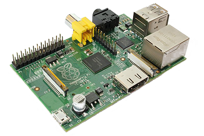
I’ve got a laptop and a Raspberry Pi, so I decided to put this to the test.
MathematicaMark
Mathematica ships with a benchmarking package called MathematicaMark. The latest version of the benchmark, MathematicaMark9, consists of 15 tests that use both numeric and symbolic functions. The MathematicaMark score is the geometric mean of the reciprocal of the timings, normalized against some reference system’s timings:
$$ \sqrt[15]{\prod_{i=1}^{15} \frac{t_{r,i}}{t_{s,i}}} $$
…where $t_{s,i}$ is the timing for test $i$ on system $s$ and $r$ is the reference system. For MathematicaMark9, the reference system is a 3.07 GHz Core i7-950 with 8 hyper-threaded cores running 64-bit Windows 7 Pro. By definition, this system has a MathematicaMark9 score of 1.0.
We can compare systems using the MathematicaMark score. If a system were 10 to 20 times slower, we would expect its MathematicaMark score to be anywhere from 1/10th to 1/20th the value of the faster system. The Benchmark[] function also provides the timings for the individual tests, so we can dig in and see which functions might be benefitting from the architecture-specific internal libraries Wolfram mentioned.
Raspberry Pi Configuration

I used a Model B Raspberry Pi with 512MB of RAM. The tests were done after a fresh install of NOOBS 1.3.3, which includes Mathematica and the Wolfram Language installed by default. wolfram was invoked from the commandline and nothing else was running on the system, most notably the X Window System and the Mathematica Notebook interface.
“Typical Current-Model Laptop”

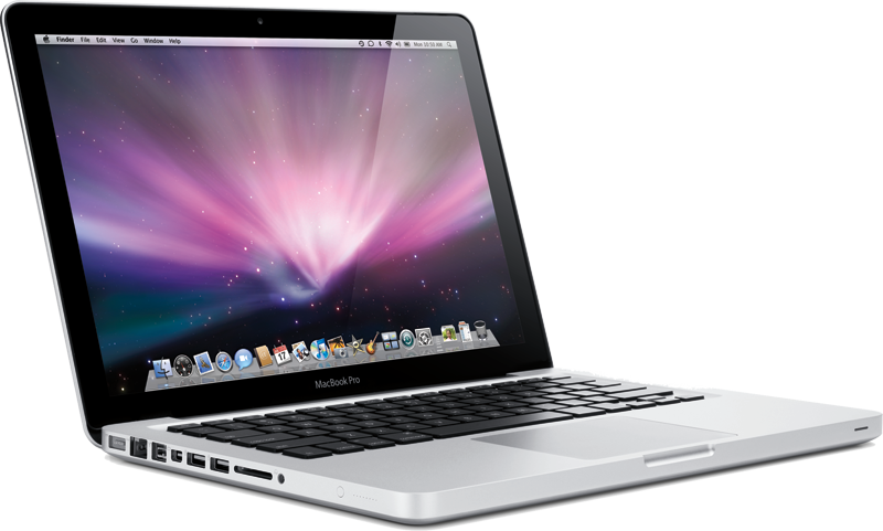
Mathematica ships with benchmark results for 15 different systems (including the reference system). It’s not clear which system to use for this comparison, so I conveniently chose my Early 2013 13-inch Retina MacBook Pro, which sports a 2.6 GHz Intel Core i5 processor (4 hyper-threaded cores) as a representative “typical current-model laptop.” Based on the sea of glowing Apple logos I’ve seen in the audiences of the conferences I attended this year, I think it’s a fair selection.
MathematicaMark9 Scores
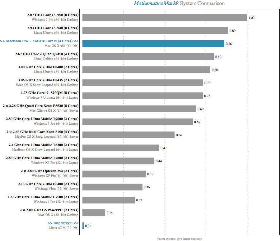
With the setup out of the way, let’s take a look at the report comparing the MacBook, Raspberry Pi, and the 15 included systems:
The MacBook Pro weighs in at a respectible 0.86, while the Raspberry Pi is actually getting rounded up to 0.01 from a true score of 0.005. Running the benchmark takes 16 seconds on the laptop and nearly 49 minutes on the Raspberry Pi.
Even the slowest machine in the included benchmarks score nearly 30x higher. I don’t think Wolfram would consider a pre-Intel Mac to be a “typical current-model” computer. To see the numbers he’s citing, we need to dig into the timings for the individual tests.
Performance on Individual Tests
The source for the 15 individual tests and the timings on a variety of reference systems is included in the full MathematicaMark9 Benchmark Report. Here are the timings on the Raspberry Pi and the Macbook Pro:
| Test | Pi Timing (s) | Mac Timing (s) | Ratio |
|---|---|---|---|
| Random Number Sort | 25.13 | 1.75 | 14.4 |
| Digits of Pi | 12.30 | 0.78 | 15.9 |
| Matrix Arithmetic | 27.76 | 1.25 | 22.2 |
| Gamma Function | 15.77 | 0.63 | 25.2 |
| Large Integer Multiplication | 19.20 | 0.58 | 32.9 |
| Polynomial Expansion | 4.55 | 0.12 | 36.4 |
| Numerical Integration | 35.41 | 0.96 | 36.7 |
| Matrix Transpose | 36.77 | 0.95 | 38.8 |
| Data Fitting | 29.94 | 0.66 | 45.4 |
| Discrete Fourier Transform | 79.28 | 0.95 | 83.4 |
| Elementary Functions | 174.93 | 1.31 | 133.3 |
| Eigenvalues of a Matrix | 136.87 | 0.79 | 174.1 |
| Singular Value Decomposition | 433.08 | 1.52 | 284.0 |
| Solving a Linear System | 745.53 | 1.65 | 452.1 |
| Matrix Multiplication | 1136.51 | 2.15 | 528.9 |
Sorting by the ratio reveals that there are definitely cases where the relative performance falls in the 10x – 20x range cited by Wolfram.
It’s interesting to note that the 4 worst performing tests by ratio are all linear algebra operations involving matrix decomposition or multiplication. These are the types of operations that have probably gotten a lot of optimization love from Wolfram Research developers in the past because this is the area that potential users compare when deciding between Mathematica and its competitors, particularly Matlab.
If you look through the revision history highlights of Mathematica, you’ll see that there was a sequence of releases where every version had at least one top-level mention of linear algebra performance improvements:
- Mathematica 5.0 – 2003
- “Record-breaking speed through processor-optimized numerical linear algebra”
- “Full support for high-speed sparse linear algebra”
- Mathematica 5.1 – 2004
- “Numerical linear algebra performance enhancements”
- Mathematica 5.2 – 2005
- “Multithreaded numerical linear algebra”
- “Vector-based performance enhancements”
The 5th worst test by ratio, Elementary Functions, is also interesting to dig into. Here’s the source:
1 2 3 4 5 6 7 8 9 10 | |
It’s computing $ e^x $, $ \sin{x} $, and $ \text{tan}^{-1} \frac{x}{y} $ for lists of 2,200,000 random numbers 30 times. Exp, Sin, and ArcTan all have the Listable attribute, which means that they are automatically mapped over lists that are passed in as arguments. Sin[list] and Map[Sin, list] are functionally equivalent, but the former provides the implementation the opportunity to take an optimized path if there is a faster way of computing the sine of multiple numbers.
We can verify that this is a case where architecture specific optimizations are in play by rewriting the test to use Map and MapThread:
1 2 3 4 5 6 7 8 | |
Note that I’m only running this once, as opposed to the 30 times in the original test, because the non-Listable version is so much slower.
The version that doesn’t take advantage of the Listable attribute takes 1.63 seconds on the Macbook Pro and 62.64 seconds on the Raspberry Pi. This ratio of 38.2 (vs. 133.3 before) is much closer to the ratio we see from the other tests that don’t take advantage of specifics of the architecture.
Conclusion
Even though Mathematica is much slower on the Raspberry Pi, it’s a tremendous free gift and it still has many uses:
A recent guest post from Wolfram Research on the Raspberry Pi blog links to several projects that take advantage of the easy ways of controlling hardware using Mathematica on the Raspberry Pi.
Much of what most people use Mathematica for doesn’t require extreme performance. For instance, getting the closed form of an integral or derivative is still practically instantaneous from a human’s perspective.
Just getting to experience the language and environment with only a $35 investment is worthwhile. For developers, there is a lot to learn from the language, which is heavily influenced by Lisp’s M-expressions, and the notebook enviroment, which is just starting to be replicated by iPython. On top of that, the incredible interactive documentation for the language is something everyone should experience.
Any questions, corrections, or suggestions are appreciated!
