A few weeks ago, I knocked my favorite mug off the counter and it shattered. RIP:
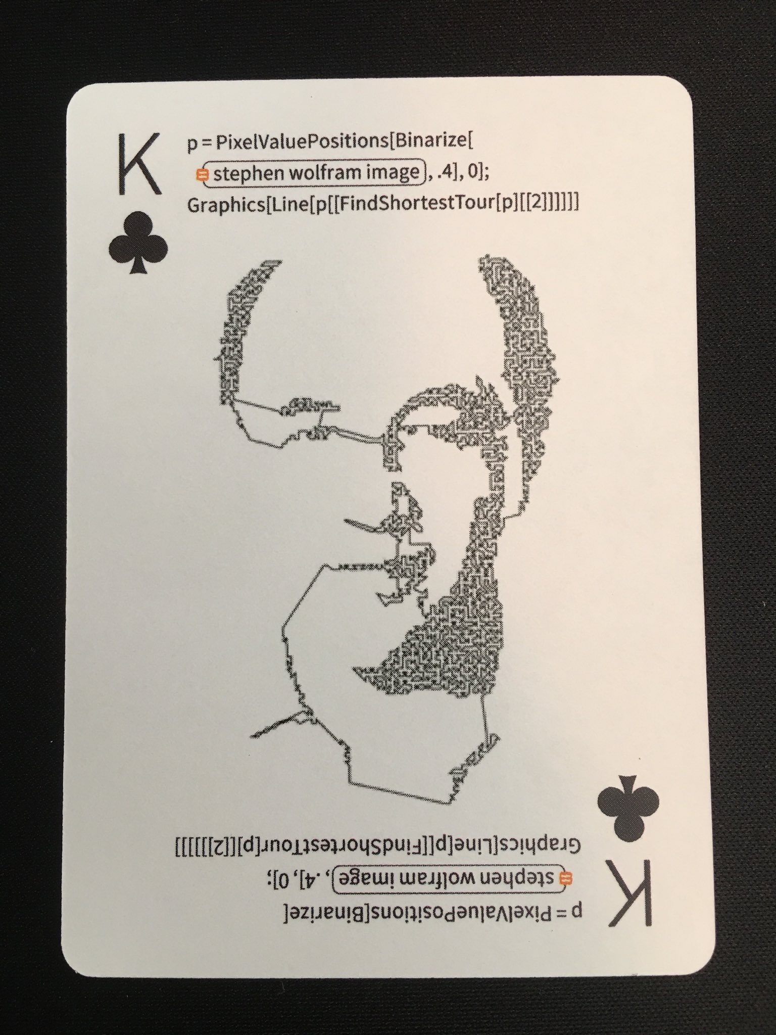
Like a good consumer, I immediately went to the Wolfram store to buy a replacement, but they no longer make it. They did have a deck of playing cards which promised a unique illustration and generating code on each card. How could I pass it up?
The cards arrived a few days ago and they were way cooler than I imagined. As I flipped through the deck, I realized a lot of the cards would be really interesting as starting points for animations. I’ve been going to town with them and posting to Twitter in an epic thread.
4♥️ (Hot take: this is surprisingly bad code. Side effects? Unnecessary call to Image in the loop? Should be a single expression!) pic.twitter.com/XsJUHM67El
Halite is a new AI programming competition that was recently released by Two Sigma and Cornell Tech. It was designed and implemented by two interns at Two Sigma and was run as the annual internal summer programming competition.
While the rules are relatively simple, it proved to be a surprisingly deep challenge. It’s played on a 2D grid and a typical game looks like this:
Each turn, all players simultaneously issue movement commands to each of their pieces:
Move to an adjacent location and capture it if you are stronger than what’s currently there.
Stay put and build strength based on the production value of your current location.
When two players’ pieces are adjacent to each other, they automatically fight. A much more detailed description is available on the Halite Game Rules page.
Bots are run as subprocesses that communicate with the game environment through STDIN and STDOUT, so it’s very simple to create bots in the language of your choice. While Python, Java, and C++ bot kits were all provided by the game developers, the community quickly produced kits for C#, Rust, Scala, Ruby, Go, PHP, Node.js, OCaml, C, and Clojure. All the starter packages are available on the Halite Downloads page.
Clojure Bot Basics
The flow of all bots are the same:
Read the initial state (your player ID and the starting game map conditions)
Write your bot’s name
Read the current gam emap
Write your moves
GOTO #3
The Clojure kit represents the game map as a 2D vector of Site records:
A simple bot that finds all the sites you control and issues random moves would look like this:
123456789101112131415161718
(ns MyBot(:require[game][io])(:gen-class))(defn random-moves"Takes your bot's ID and a 2D vector of Sites and returns a map from site to direction"[my-idgame-map](let [my-sites(->>game-mapflatten(filter #(= (:owner%)my-id)))](zipmap my-sites(repeatedly#(rand-nthgame/directions)))))(defn -main[](let [{:keys[my-idproductionswidthheightgame-map]}(io/get-init!)](println "MyFirstClojureBot")(doseq [turn(range)](let [game-map(io/create-game-mapwidthheightproductions(io/read-ints!))](io/send-moves!(random-movesmy-idgame-map))))))
I recently gave a talk on the Bag of Little Bootstraps algorithm at Papers We Love Too in San Francisco:
My part starts around 31:27, but you should watch the excellent mini talk at the beginning too! For reference, here are all the papers that are mentioned in the talk:
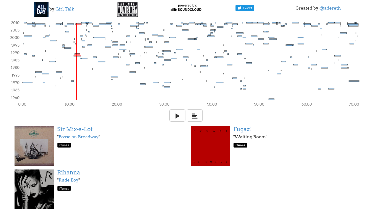
Greg Gillis, also known as Girl Talk, is an impressive DJ who creates mega-mashups consisting of hundreds of samples. His sample selections span 7 decades and dozens of genres. Listening to his albums is a bit like having a concentrated dump of music history injected right into your brain.
I became a little obsessed with his work last year and I wanted a better way to experience his albums, so I created an annotated player using Clojure and d3 that shows relevant data and links about every track as it plays:
I have versions of this player for his two most recent albums:
Unfortunately, they only really work on the desktop right now.
Parsing Track Data
I’ve released all the code that I used to collect the data and to generate the visualizations, but in this post I’m just going to talk about the first stage of the process: getting the details of which tracks were sampled at each time.
There’s an excellent (totally legal!) crowd-sourced wiki called Illegal Tracklist that has information about most of the samples displayed like this:
At first, I used Enlive to suck down the HTML versions of the wiki pages, but I realized it might be cleaner to operate off the raw wiki markup which looks like this:
I wrote a few specialized functions to pull the details out of the strings and into a data structure, but it quickly became unwieldy and unreadable. I then saw that this was a perfect opportunity to use Instaparse. Instaparse is a library that makes it easy to build parsers in Clojure by writing context-free grammars.
Here’s the Instaparse grammar that I used that parses the Illegal Tracklists’ markup format:
The high level structure is practically self-documenting: each line in the wiki source is either a title track line, a sample track line, or a blank line and each type of line is pretty clearly broken down into named components that are separated by string literals to be ignored in the output. It does, however, become a bit nasty when you get to the terminal rules that are defined as regular expressions. Instaparse truly delivers on its tagline:
What if context-free grammars were as easy to use as regular expressions?
The only problem is that regular expressions aren’t always easy to use, especially when you have to start worrying about not greedily matching the text that is going to be used by Instaparse.
Some people, when confronted with a problem, think “I know, I'll use Instaparse.” Now they have three problems. #clojure
Despite some of the pain of regular expressions and grammar debugging, Instaparse was awesome for this part of the project and I would definitely use it again. I love the organization that it brought to the code and the structure I got out was very usable:
I did the entire presentation as one huge sequence of animations using D3.js. The Youtube video doesn’t capture the glory that is SVG, so I’ve posted the slides.
I also finally got to apply the technique that I wrote about in my Colorful Equations with MathJax post from over a year ago, only instead of coloring explanatory text, the colors in the accompanying chart match:
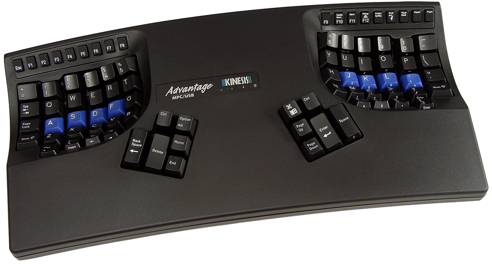
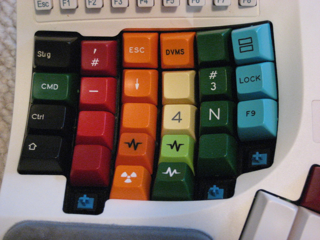
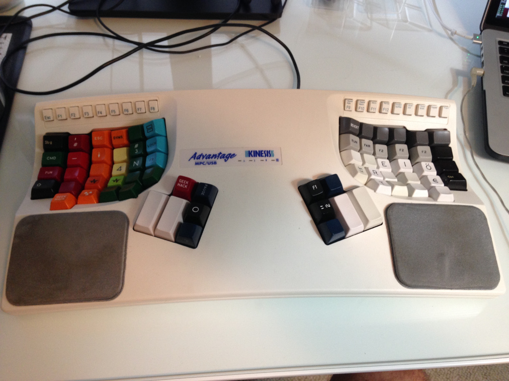
I’ve been (slowly) working on building my own dream keyboard, but in the meantime I make the occasional ridiculous tweak to my Kinesis. This weekend I got 3 lbs. of reject keys from Signature Plastics and I was fortunate enough to get enough keycaps to try something that I’ve been wanting to test for a while.
They are particularly well suited for non-standard keyboard layouts, like the ErgoDox or Kinesis Advantage, because most other keycaps have variable heights and angles that were designed for traditional staggered layouts on a plane.
SA keycaps
Personally, I’m a big fan of the SA profile:
They’re super tall and are usually manufactured with thick ABS plastic and given a smooth, high-gloss finish. I’m a bit of a retro-fetishist and these hit all the right spots. It’s no surprise that projects and group buys that use SA profile often have a retro theme:
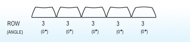
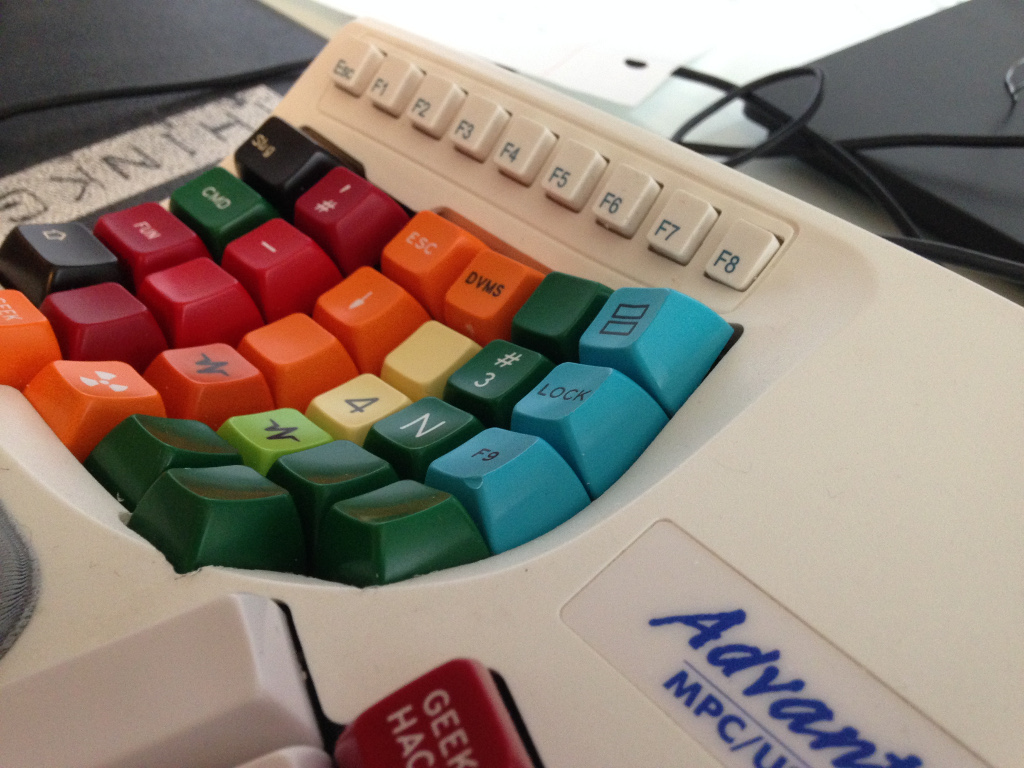
For this project I decided to go with all Row 3 profile SA keys in the two main key wells. Row 3 is the home row on traditional layouts and the keycaps are completely symmetric, just like the DSA profile keys. I was concerned about two main things:
The curvature of the key well combined with the height might mean that the keys hit each other towards the top.
Jesse ran into one spot in the corner of the keywell closest to the thumb clusters where the keycap hit the plastic. This would almost certainly be a problem with the much larger SA keys.
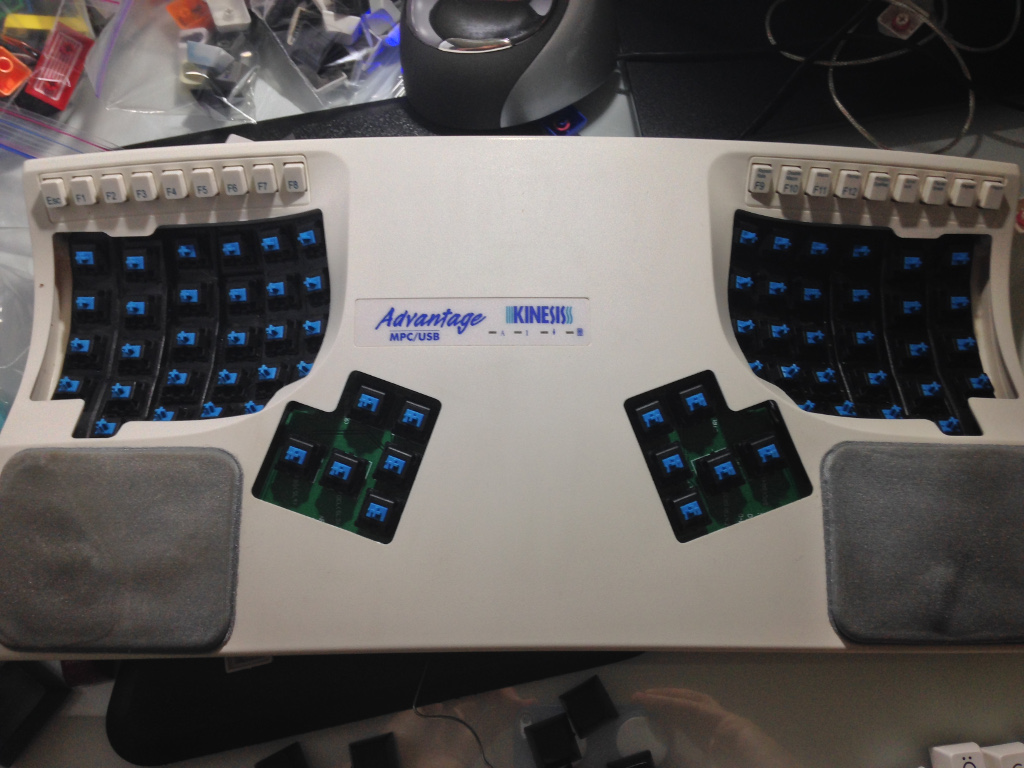
The easiest way to find out was to pop off all the keycaps:
…and to see what fit:
Fortunately, the height was not an issue. The angles are all perfect and the top of the keys form a relatively tight surface. The smaller gaps between the tops combined with the extreme smoothness of the SA keycaps results in a nice effect where I’m able to just glide my fingers across them without having to lift, similar to the feel of the modern Apple keyboards.
Unfortunately, 3 keys at the bottom of each keywell wouldn’t fit. I busted out the Dremel and carved out a little from the bottom, making room for those beautiful fat caps:
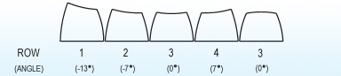
I used Row 1 keycaps for the 1x keys in the thumb clusters. The extra height makes them not quite as difficult to reach:
Conclusion
Overall, I’m pretty happy with how it turned out:
It’s a pleasure to type on and I’m convinced that SA profile keys are going to be what I use when I eventually reach my final form.
If you’re interested in doing this yourself, you should know that it’ll be difficult to source the 1.25x keys that are used on the sides of the Kinesis Advantage. A lot of the keysets that are being sold for split layouts are targeting the Ergodox, which uses 1.5x keys on the side. It does look like the Symbiosis group buy includes enough 1.25x’s in the main deal, but you’d need to also buy the price Ergodox kit just to get those 4 2x’s. If you don’t mind waiting an indefinite length of time, the Round 5a group buy on Deskthority is probably your best bet for getting exactly what you want.
I recently started learning about Algebraic Lattices because I was interested in how they relate to Automata Theory. It turns out they’re fundamental to a bunch of other things that I’ve always wanted to learn more about, like CRDTs and Type Theory.
I stumbled upon an interesting property about lattices that reminded me of something from Graph Theory…
If $(L, \leq)$ is a partially ordered set, and $S \subseteq L$ is an arbitrary subset, then an element $u \in L$ is said to be an upper bound of $S$ if $s \leq u$ for each $s \in S$. A set may have many upper bounds, or none at all. An upper bound $u$ of $S$ is said to be its least upper bound, or join, or supremum, if $u \leq x$ for each upper bound $x$ of $S$. A set need not have a least upper bound, but it cannot have more than one. Dually, $l \in L$ is said to be a lower bound of $S$ if $l \leq s$ for each $s \in S$. A lower bound $l$ of $S$ is said to be its greatest lower bound, or meet, or infimum, if $x \leq l$ for each lower bound $x$ of $S$. A set may have many lower bounds, or none at all, but can have at most one greatest lower bound.
A partially ordered set $(L, \leq)$ is called a join-semilattice and a meet-semilattice if each two-element subset $\{a,b\} \subseteq L$ has a join (i.e. least upper bound) and a meet (i.e. greatest lower bound), denoted by $a \vee b$ and $a \wedge b$, respectively. $(L, \leq)$ is called a lattice if it is both a join- and a meet-semilattice.
That’s a lot to take in, but it’s not so bad once you start looking at lattices using Hasse diagrams. A Hasse diagram is a visualization of a partially ordered set, where each element is drawn below the other elements that it is less than. Edges are drawn between two elements $x$ and $y$ if $x < y$ and there is no $z$ such that $x < z < y$.
For example, if we define the $\leq$ operator to be “is a subset of”, we get a partial ordering for any powerset. Here’s the Hasse diagram for the lattice $(\mathcal{P}(\{1,2,3\}), \subseteq)$:
In this case, the $\subseteq$ operator results in $\vee$ (the “join”) being union of the sets and $\wedge$ (the “meet”) as the intersection of the sets. It’s a tragic failure of notation that $\vee$ means you should find the common connected element that is above the pair in the diagram and $\wedge$ means you should look below.
Another example is the set of divisors of a number, where the $\leq$ operator means “divides into”. Here’s the Hasse diagram for all the divisors of 30:
In this case, $\vee$ ends up meaning Least Common Multiple and $\wedge$ means Greatest Common Divisor.
Yet another example is the set of binary strings of a fixed length $n$, with $S \leq T$ meaning $S_i \leq T_i$ for $1 \leq i \leq n$:
In this case, $\vee$ is the binary OR operator and $\wedge$ is the binary AND operator.
These examples are interesting because they’re all the same structure! If we can prove a fact about the structure, we get information about all three systems. These happen to be Boolean lattices, which have the distributive property:
$$a \vee (b \wedge c) = (a \vee b) \wedge (a \vee c)$$
$$\forall a, b, c \in L$$
Now here’s the neat part. There are fundamentally only two lattices that aren’t distributive:
The Diamond Lattice
$$a \vee (b \wedge c) \stackrel{?}{=} (a \vee b) \wedge (a \vee c)$$
$$a \vee 0 \stackrel{?}{=} 1 \wedge 1$$
$$a \neq 1$$
…and:
The Pentagon Lattice
$$a \vee (b \wedge c) \stackrel{?}{=} (a \vee b) \wedge (a \vee c)$$
$$a \vee 0 \stackrel{?}{=} 1 \wedge c$$
$$a \neq c$$
Any lattice that has a sub-lattice that is isomorphic to either the Diamond or Pentagon, referred to as $M_3$ and $N_5$ respectively, is not distributive. It’s not too hard to see, just verify that the corresponding elements that violate distribution above will fail no matter what else is going on in the lattice.
The surprising part is that every non-distributive lattice must contain either $M_3$ or $N_5$! In a sense these are the two poisonous minimal shapes: their presence kills distributivity.
This alone seems like a cool little fact, but what struck me was that this isn’t the first time that I’ve seen something like this…
Planar Graphs
In Graph Theory, there’s a property of graphs called planarity. If you can draw the graph without any of the edges crossing, the graph is planar. The Wikipedia page on planar graphs is filled with awesome facts. For example, a planar graph can’t have an average degree greater than 6 and any graph that can be drawn planarly with curvy edges can be drawn planarly with straight edges, but the most famous result concerning planar graphs is Kuratowski’s Theorem:
A finite graph is planar if and only if it does not contain a subgraph that is a subdivision of $K_5$ (the complete graph on five vertices) or of $K_{3,3}$ (the complete bipartite graph on six vertices)
$K_5$, the complete graph on five vertices
$K_{3,3}$, the complete bipartite graph on six vertices
It turns out there are fundamentally only two graphs that aren’t planar! Any graph that “contains” either of these two graphs is not planar and any graph that isn’t planar must “contain” one of them. The meaning of “contains” is a little different here. It’s not enough to just find vertices that form $K_5$ or $K_{3,3}$ with the edges that connect them. What we need to check is if any subgraph can be “smoothed” into one of these two graphs.
For example, this graph isn’t planar because the red vertex can be smoothed away, leaving $K_{3,3}$:
And?
Unfortunately, I’m just learning about lattice theory and I have no idea if there’s any formal connection between these similar concepts. I have found that there is a branch of lattice theory that is concerned with the planarity of the Hasse diagrams, so it’s not like any algebraist hasn’t thought of this before. If anyone has a formal connection or an example of other cases where a pair of structures have this kind of “poisonous” property, I’d love to hear.
You might be interested in the Robertson-Seymour theorem which says that for any graph property that is closed under taking minors there is a finite list of “forbidden minors” or as you call them “poisonous” graphs. Kuratowski’s theorem is one particular example of this.
This relates also to the concept of well-quasi-orders. A quasi-ordered set $(X, \leq)$ is a well-quasi-order if every infinite sequence ($x_1, x_2, …$) with elements in $X$ has some $i < j$ with $x_i \leq x_j$. An equivalent statement of the Robertson-Seymour theorem is that the set of all finite graphs ordered by the minor relation is well-quasi-ordered.
Another example where “forbidden minors” appear is matroids. Matroids also have minors but unlike graphs they are not well-quasi-ordered under the minor relation. However certain minor closed properties do have a finite list of forbidden minors. For example Rota’s conjecture, which was announced to be proven very recently, says that for any finite field the set of matroids that are representable over that field are characterized by a finite list of forbidden minors.
I started digging into the history of mode detection after watching Aysylu Greenberg’s Strange Loop talk on benchmarking. She pointed out that the usual benchmarking statistics fail to capture that our timings may actually be samples from multiple distributions, commonly caused by the fact that our systems are comprised of hierarchical caches.
I thought it would be useful to add the detection of this to my favorite benchmarking tool, Hugo Duncan’s Criterium. Not surprisingly, Hugo had already considered this and there’s a note under the TODO section:
12
Multimodal distribution detection.
Use kernel density estimators?
I hadn’t heard of using kernel density estimation for multimodal distribution detection so I found the original paper, Using Kernel Density Estimates to Investigate Multimodality (Silverman, 1981). The original paper is a dense 3 pages and my goal with this post is to restate Silverman’s method in a more accessible way. Please excuse anything that seems overly obvious or pedantic and feel encouraged to suggest any modifications that would make it clearer.
What is a mode?
The mode of a distribution is the value that has the highest probability of being observed. Many of us were first exposed to the concept of a mode in a discrete setting. We have a bunch of observations and the mode is just the observation value that occurs most frequently. It’s an elementary exercise in counting. Unfortunately, this method of counting doesn’t transfer well to observations sampled from a continuous distribution because we don’t expect to ever observe the exact some value twice.
What we’re really doing when we count the observations in the discrete case is estimating the probability density function (PDF) of the underlying distribution. The value that has the highest probability of being observed is the one that is the global maximum of the PDF. Looking at it this way, we can see that a necessary step for determining the mode in the continuous case is to first estimate the PDF of the underlying distribution. We’ll come back to how Silverman does this with a technique called kernel density estimation later.
What does it mean to be multimodal?
In the discrete case, we can see that there might be undeniable multiple modes because the counts for two elements might be the same. For instance, if we observe:
$$1,2,2,2,3,4,4,4,5$$
Both 2 and 4 occur thrice, so we have no choice but to say they are both modes. But perhaps we observe something like this:
$$1,1,1,2,2,2,2,3,3,3,4,9,10,10$$
The value 2 occurs more than anything else, so it’s the mode. But let’s look at the histogram:
That pair of 10’s are out there looking awfully interesting. If these were benchmark timings, we might suspect there’s a significant fraction of calls that go down some different execution path or fall back to a slower level of the cache hierarchy. Counting alone isn’t going to reveal the 10’s because there are even more 1’s and 3’s. Since they’re nestled up right next to the 2’s, we probably will assume that they are just part of the expected variance in performance of the same path that caused all those 2’s. What we’re really interested in is the local maxima of the PDF because they are the ones that indicate that our underlying distribution may actually be a mixture of several distributions.
Kernel density estimation
Imagine that we make 20 observations and see that they are distributed like this:
We can estimate the underlying PDF by using what is called a kernel density estimate. We replace each observation with some distribution, called the “kernel,” centered at the point. Here’s what it would look like using a normal distribution with standard deviation 1:
If we sum up all these overlapping distributions, we get a reasonable estimate for the underlying continuous PDF:
Note that we made two interesting assumptions here:
We replaced each point with a normal distribution. Silverman’s approach actually relies on some of the nice mathematical properties of the normal distribution, so that’s what we use.
We used a standard deviation of 1. Each normal distribution is wholly specified by a mean and a standard deviation. The mean is the observation we are replacing, but we had to pick some arbitrary standard deviation which defined the width of the kernel.
In the case of the normal distribution, we could just vary the standard deviation to adjust the width, but there is a more general way of stretching the kernel for arbitrary distributions. The kernel density estimate for observations $X_1,X_2,…,X_n$ using a kernel function $K$ is:
Note that changing $h$ has the exact same effect as changing the standard deviation: it makes the kernel wider and shorter while maintaining an area of 1 under the curve.
Different kernel widths result in different mode counts
The width of the kernel is effectively a smoothing factor. If we choose too large of a width, we just end up with one giant mound that is almost a perfect normal distribution. Here’s what it looks like if we use $h=5$:
Clearly, this has a single maxima.
If we choose too small of a width, we get a very spiky and over-fit estimate of the PDF. Here’s what it looks like with $h = 0.1$:
This PDF has a bunch of local maxima. If we shrink the width small enough, we’ll get $n$ maxima, where $n$ is the number of observations:
The neat thing about using the normal distribution as our kernel is that it has the property that shrinking the width will only introduce new local maxima. Silverman gives a proof of this at the end of Section 2 in the original paper. This means that for every integer $k$, where $1<k<n$, we can find the minimum width $h_k$ such that the kernel density estimate has at most $k$ maxima. Silverman calls these $h_k$ values “critical widths.”
Finding the critical widths
To actually find the critical widths, we need to look at the formula for the kernel density estimate. The PDF for a plain old normal distribution with mean $\mu$ and standard deviation $\sigma$ is:
For a given $h$, you can find all the local maxima of $\hat{f}$ using your favorite numerical methods. Now we need to find the $h_k$ where new local maxima are introduced. Because of a result that Silverman proved at the end of section 2 in the paper, we know we can use a binary search over a range of $h$ values to find the critical widths at which new maxima show up.
Picking which kernel width to use
This is the part of the original paper that I found to be the least clear. It’s pretty dense and makes a number of vague references to the application of techniques from other papers.
We now have a kernel density estimate of the PDF for each number of modes between $1$ and $n$. For each estimate, we’re going to use a statistical test to determine the significance. We want to be parsimonious in our claims that there are additional modes, so we pick the smallest $k$ such that the significance measure of $h_k$ meets some threshold.
Bootstrapping is used to evaluate the accuracy of a statistical measure by computing that statistic on observations that are resampled from the original set of observations.
Silverman used a smoothed bootstrap procedure to evaluate the significance. Smoothed bootstrapping is bootstrapping with some noise added to the resampled observations. First, we sample from the original set of observations, with replacement, to get $X_I(i)$. Then we add noise to get our smoothed $y_i$ values:
Where $\sigma$ is the standard deviation of $X_1,X_2,…,X_n$, $h_k$ is the critical width we are testing, and $\epsilon_i$ is a random value sampled from a normal distribution with mean 0 and standard deviation 1.
Once we have these smoothed values, we compute the kernel density estimate of them using $h_k$ and count the modes. If this kernel density estimate doesn’t have more than $k$ modes, we take that as a sign that we have a good critical width. We repeat this many times and use the fraction of simulations where we didn’t find more than $k$ modes as the p-value. In the paper, Silverman does 100 rounds of simulation.
One of the biggest weaknesses in Silverman’s technique is that the critical width is a global parameter, so it may run into trouble if our underlying distribution is a mixture of low and high variance component distributions. For an actual implementation of mode detection in a benchmarking package, I’d consider using something that doesn’t have this issue, like the technique described in Nonparametric Testing of the Existence of Modes (Minnotte, 1997).
I hope this is correct and helpful. If I misinterpreted anything in the original paper, please let me know. Thanks!
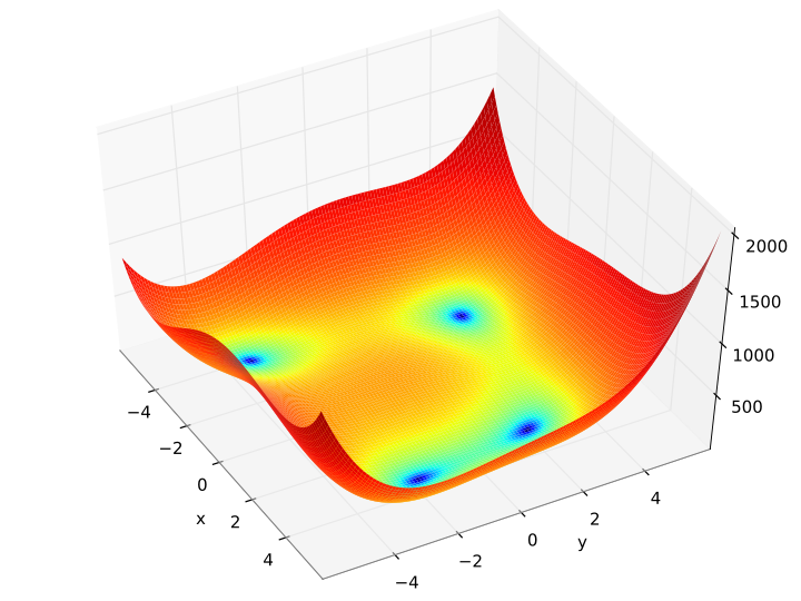 Himmelblau’s Function, a popular test function for black-box optimization


